20Q: Frequency Lowering Ten Years Later - New Technology Innovations

From the Desk of Gus Mueller

A lot can change in 10 years in the world of technology. Consider that in 2006, Twitter was just birthed and only known to a handful of people, the first iPhone had yet to be introduced, and Uber hadn’t even been founded.  Things don’t explode quite as fast in the world of hearing aids, but a technology that was around in 2006 was frequency lowering—the modern version of which was introduced that year by Widex. One by one, over the years that have followed, other companies have introduced their version of frequency lowering, and today this technology is available from all major manufacturers.  

The adoption rate of frequency lowering among audiologists has been interesting. It has been embraced by some, who fit it to the majority of their patients.  Others have never activated this processing for any of their patients. And there are probably a few, who are fitting frequency lowering and don’t even know it, as they are not carefully observing the software default settings.

Like most hearing aid technology, maximizing the effectiveness of frequency lowering requires a good understanding of how the algorithm works, how it can be adjusted, what has to be done to individualize it for a given patient, and of course, the use of some verification procedure that confirms that the changes have resulted in an optimum fitting. Four basic steps that we reviewed here at AudiologyOnline a few years ago, when Josh Alexander, Susan Scollie and I published a series of three articles on frequency lowering titled, The Highs and Lows, The Ins and Outs, and The Whole Shebang.

Three years have passed since our frequency-lowering trilogy. Has anything changed? You bet! There are new products, and new revisions of the algorithms of some of the older products.  And who better to talk about all this than one of our frequency-lowering gurus of three years ago, Josh Alexander.

Joshua M. Alexander, PhD, is Assistant Professor, Department of Speech, Language, & Hearing Sciences, Purdue University, and the Director of the Purdue Experimental Amplification Research (EAR) Laboratory (check out TinyURL.com/PurdueEAR). You are probably familiar with his many publications relating to the auditory processes contributing to speech perception deficits in hearing-impaired listeners, and the hearing aid signal processing strategies that can be used to overcome them. He is a frequently requested speaker on these topics at professional meetings.

Relating to our 20Q topic this month, Dr. Alexander’s research efforts have led to the development of a hearing aid simulator; a key element of this simulator is an algorithm for nonlinear frequency compression.  His work in this area has led to one patent in place, a separate patent application submitted, and two disclosures, one in the area of speech enhancement for human and machine processing and one concerning frequency lowering.

It’s naturally expected that when you ask an expert to talk about his favorite topic, you’re going to get a sizeable amount of information.  That’s a good thing.  You’ll see in this excellent 20Q that Josh goes into many of the details and fine points that clinicians need to know when fitting frequency lowering.  It’s probably not something you can skim through—but why would you want to?

Gus Mueller, PhD
Contributing Editor
September 2016

To browse the complete collection of 20Q with Gus Mueller CEU articles, please visit www.audiologyonline.com/20Q

20Q: Frequency Lowering Ten Years Later - New Technology Innovations
 

 Joshua Alexander

1. Since all the initial hoopla, I really haven’t paid too much attention to frequency lowering in hearing aids.  Has much really changed?

Most certainly.  You might recall that back in the 1990s, AVR Sonovation had a frequency lowering analog device, but the modern products we know today were not introduced until ten years ago.  In 2006, Widex introduced “Audibility Extender,” which was later followed by Phonak’s SoundRecover in 2008; this is when frequency lowering in its modern form started to become mainstream.  By the time we first talked about this on the pages of 20Q in 2013 (Alexander, 2013b; Scollie, 2013; Mueller, Alexander, & Scollie, 2013), Starkey and Siemens had added a frequency lowering feature to their portfolio.  Now, each of the ‘Big Six’ hearing aid manufacturers have a frequency lowering feature.  The early players, Widex and Phonak, have introduced updates to their original frequency lowering algorithms.  My guess is that the rest of the players are actively working on updates to their algorithms as well.  There is a lot to keep track of when making comparisons between the different methods, and most discussions on the matter necessarily require references to abstract concepts.  Therefore, to help you understand the differences we will be talking about, I have created a series of online tools that I call Frequency Lowering Fitting Assistants that show how the frequencies picked up at the input to the hearing aid microphone are lowered at the output of the hearing aid receiver.  These fitting assistants are available at my lab's website, and can be accessed at: www.tinyURL.com/FLassist.

2. What do you mean by "frequency lowering in its modern form?"

Most, but not all, of the experimental frequency lowering algorithms in the published literature from the 1950s to the 1990s used one of two approaches. One approach was a form of transposed vocoding, which is using a narrowband of low-frequency noise to synthesize the time-varying amplitude of a high-frequency band centered in the range where voiceless fricatives tend to have most of their energy.  The other approach compressed the entire frequency spectrum available at the input of the microphone, like the method utilized in AVR Sonovation’s products (see Simpson, 2009).  These techniques were limited in their effectiveness due to things like processing artifact, and so were often targeted to those with severe to profound hearing loss who had a very limited bandwidth of audibility.  The key differentiators between these earlier methods and the methods now implemented by the Big Six are that modern methods are all digital and they only lower a portion of the speech spectrum instead of the entire range.

3. What are the advantages of being able to lower only a portion of the frequency range?

The real advantages are that the low and mid frequencies that are already audible without lowering do not need to be altered, or at least altered as much.  This helps preserve overall sound quality and reduces the risk of negatively affecting the perception of those speech sounds whose primary cues are in this frequency range, especially vowels (e.g., Alexander, 2016a).

4. OK, I get it.  So what really has changed since you and your colleagues published ‘The Whole Shebang’ 20Q article in 2013?

Widex and Phonak now have newer versions of their original frequency lowering algorithms and ReSound and Oticon now have frequency lowering features in their hearing aids.  Table 1 summarizes the frequency lowering methods available by each of the Big Six manufacturers and their sister companies.  The methods that are new since our 2013 series are shaded in gray.  The biggest changes are Phonak SoundRecover2 and Oticon Speech Rescue.

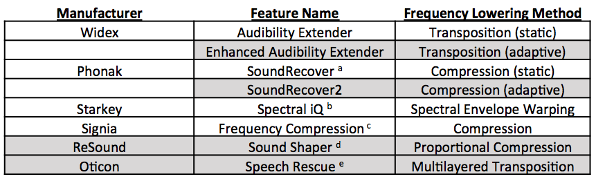
Table 1.  For each of the Big Six hearing aid corporations, the name of their frequency lowering feature and a brief description of the underlying method are provided.  Footnotes indicate the feature names used by the other companies in the same parent company as the ones listed.  The methods with a shaded background are the ones that are new since our last 20Q article series in 2013. Since our last article, Siemens has become Signia.

^a Also offered by Unitron as “Frequency Compression” and by Hansaton as "Sound Restore"

^b Also offered by Microtech as “Sound Compression”

^c Also offered by Rexton as “Bandwidth Compression”

^d Also offered by Beltone as “Sound Shifter” and by Interton as “Frequency Shifter”

^e Similar to, but not the same as, what is offered by Bernafon as “Frequency Composition” and by Sonic as “Frequency Transfer"

5. Can you briefly remind me how those methods we talked about last time work?

Sure, let’s start from the top of Table 1.  The original Audibility Extender and the newer version found in Widex hearing aids uses frequency transposition.  Audibility Extender continually searches for the most intense peak in the source region (the frequency range subject to lowering) and then copies (transposes) it down to the destination region (the frequency range where the newly-lowered information is moved to) by a linear factor of 1/2 (one octave).  The peak is band-pass filtered so that it only spans one octave after lowering.  One advantage of this filtering is that the lowered information does not need to be compressed.  This fact along with the linear downward shift helps to ensure that the harmonics of the lowered source align with the harmonics of the signal already present in the destination region.  The expanded mode of Audibility Extender has a second source region that overlaps with the first.  The destination region for this information is computed using a linear factor of 1/3 instead of 1/2 (Figure 1).

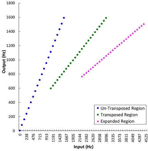
Figure 1.  Plot showing how the frequencies at the input of the hearing aid are altered at the output by Widex’s Audibility Extender.  The un-transposed signal (blue circles) is low-pass filtered above the start frequency (1600 Hz in this example), but this frequency can now be optionally changed with the new Enhanced Audibility Extender.  The transposed signal (green squares) overlaps with the un-transposed signal and is the result of lowering the input frequencies by 1/2 (one octave).  Likewise, the expanded transposed signal (magenta triangles) overlaps with the transposed signal and is the result of lowering the input frequencies by 1/3.  Source: Audibility Extender Fitting Assistant v2.0.

6. What makes the Widex Enhanced Audibility Extender different from the original version?

Kuk and colleagues (2015) identify three main enhancements to the Widex frequency lowering algorithm.  The first is a voicing detector that tries to classify the incoming high frequency signal (namely, speech) as having a harmonic or a noisy spectrum.  The glottal vibration that provides the source for voiced phonemes, like /z/ and /Θ/, results in a harmonic spectrum with lower intensity and shorter duration compared with the noisy turbulence that provides the source for voiceless phonemes, like /s/, /θ/, and /ʃ/ (Jongman, Wayland, & Wong, 2000).  Respecting these acoustic differences, the Enhanced Audibility Extender applies less gain to the lowered signal when it detects a voiced phoneme compared with a voiceless phoneme.  In addition to preserving a possible perceptual cue, the idea behind this manipulation is to prevent the lowered voiced phonemes from being distracting while maintaining saliency for the voiceless phonemes (Kuk et al., 2015).  This signal-dependent feature is the reason why I use the term “adaptive” to differentiate the new Enhanced Audibility Extender from the original “static” Audibility Extender.  As seen in Table 1, I also use this distinction for Phonak’s latest update to their frequency lowering algorithm.  Perhaps, we are seeing a trend toward adaptive frequency lowering because the processing power of the chips in the hearing aids have advanced so much that signal processing artifacts, throughput delay, current drain, etc., are not as much a concern for frequency-lowering algorithms as they once were (see Alexander 2016b for a discussion on these topics).

The second enhancement to Audibility Extender is a ‘harmonic tracking system’ that is used to help keep the harmonics of the voiced phonemes after lowering in alignment with the harmonics already present in the destination region (Kuk et al., 2015).  In theory, this should result in a more pleasant sound quality.  The third major change to Audibility Extender is the option to select the bandwidth of the original, un-lowered signal after it is mixed with lowered signal.  With the original Audibility Extender, the bandwidth of the amplified signal was low-pass filtered above the start frequency (the highest frequency in the destination region; see Alexander, 2013a,b for a more in-depth description of this terminology).  The advantage of being able to keep the bandwidth of the original signal high is that the clinician has more options for setting the source/destination regions without having to worry about artificially reducing the audible bandwidth and thereby negatively affecting speech perception.

7. Let’s jump to Starkey's approach for a moment.  I thought it was some kind of transposition, but in your chart you are calling it ‘spectral envelope warping.’  Is this the same?

The frequency lowering method implemented in Starkey hearing aids, Spectral iQ, is akin to transposition in that only a portion of the high frequency spectrum is translated down without compression.  The reason it is called ‘spectral envelope warping’ is that high frequency peaks are synthesized at lower frequencies by simply increasing the energy already present in the destination region (Galster, 2015).  Therefore, the exact nature of the output signal depends on both the low and high frequency energy present in the original signal.  As with all of the other transposition techniques on the list, the relative gain of lowered signal can be adjusted independently of the gain for the signal originally present in the destination region.  The destination region occupies a range that is approximately 500-2000 Hz wide and depends on the patient’s audiogram and the Spectral iQ Bandwidth setting (Galster, 2015).  The lowest possible frequency of the destination region corresponds to the audiometric frequency that starts the audiometric slope (preferably, 20 dB/octave or greater; see Galster 2015 for more information).  The highest possible frequency corresponds to estimated frequency where thresholds begin to exceed 70 dB HL.  There are seven settings for Spectral iQ Bandwidth: a setting of 7 corresponds to the strongest setting wherein the destination region occupies all or most of the region defined above; a setting of 1 corresponds to the weakest setting wherein the destination and source regions occupy only the upper part of the allowable frequency range.  Figure 3 demonstrates the effects of Spectral iQ and of the Bandwidth setting for a particular audiogram (Figure 2).

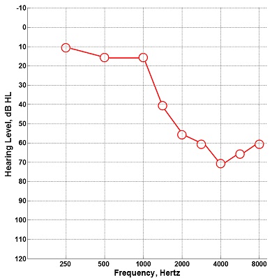
Figure 2.  Audiogram entered into the Starkey Inspire programming software that was used to evaluate the effects of Spectral iQ and changes in the Bandwidth setting as shown in Figure 3.  The allowable destination region is governed by the audiometric frequency that starts the audiometric slope (1500 Hz in this example) and the lowest frequency where thresholds are ≥ 70 dB HL (4000 Hz in this example).

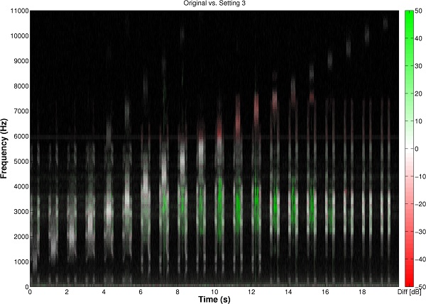
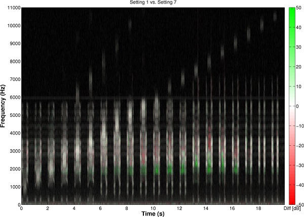
Figure 3.  Left image: For the audiogram in Figure 2, a comparative spectrogram showing the output with Starkey’s Spectral iQ algorithm activated (Bandwidth setting = 3) relative to the output with it deactivated.  The test signal consisted of natural recordings of /uʃu/, /aʃa/, /asa/, and /isi/ in which the fricative was replaced with a narrowband noise from 1000 to 10,500 Hz, in 500-Hz increments at a rate of one per second.  Where the spectrogram is white, there is no difference between the output with Spectral iQ activated and the output with it deactivated.  Where it is red, there is a loss of energy with Spectral iQ activated compared to with it deactivated.  Where it is green, there is new energy with Spectral iQ activated and it represents the lowered signal.  Notice that lowering in this example does not begin until the energy in the input band begins to exceed about 5000 Hz and that the destination region is between about 2000-4000 Hz.  Notice also that Spectral iQ will maintain the original source spectrum up to 5700 Hz (white bands) in order to provide a fuller spectrum of sound for users with aided audibility above the destination region (just as is now the option with the Widex Enhanced Audibility Extender).  The upper two channels are turned off when Spectral iQ is on (red bands at and above 6000 Hz).  The highest frequency lowered by Spectral iQ is about 9000 Hz.  Right image:  For the audiogram in Figure 2, a comparative spectrogram showing the output with Spectral iQ Bandwidth setting = 1, relative to Spectral iQ Bandwidth setting = 7.  Where the spectrogram is red there is more energy with Spectral iQ Bandwidth setting = 1, and where it is green there is more energy with Spectral iQ Bandwidth setting = 7.  The effect of changing the setting from 1 to 7 is to expand and/or shift the destination region lower in frequency (1500 Hz, in this example).

8. So how does the Starkey approach compare to the transposition technique in Oticon’s new Speech Rescue algorithm?

First, the term transposition is used for Oticon's Speech Rescue because, like Widex’s Audibility Extender, information in the source region is shifted down, without compression, to the destination region by a fixed amount.  In addition, the clinician has the option to maintain the gain of the frequencies above the destination region in order to ensure that aided bandwidth is not negatively affected by his/her choice of Speech Rescue configuration.  This is similar in concept to both Starkey’s algorithm and Widex’s new algorithm.  However, this is where the similarities end.  One difference among the methods is that Oticon Speech Rescue divides the source region into two or three sub-regions. There are three sub-regions for Speech Rescue Configuration numbers 1 to 5 and two sub-regions for Configuration numbers 6 to 10 (for more details about the Speech Rescue settings, see Angelo, Alexander, Christiansen, Simonsen, & Jespersgaard, 2015).  The sub-regions are then linearly shifted down, but not by integer ratios.  Instead, as shown in Figure 4, they are each shifted in a way that they become superimposed or layered in the destination region; hence the term “multilayered transposition” in Table 1.  The rationale for this approach is that a wide range of frequencies from the input can be represented in a narrow region in the output.  One advantage of keeping the destination region narrow is that disruption of existing low frequency information in the destination region is minimized, especially if a configuration is chosen that places the destination band near the edge of the range of aided audibility.  Another advantage is that the cochlear distance spanned by the destination region is not too much shorter than that spanned by the source region.

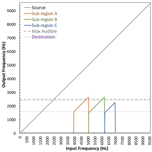
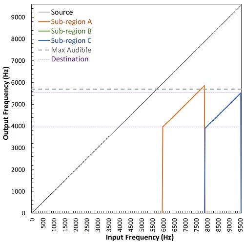
Figure 4.  Plots showing the multilayered transposition method of frequency lowering used by Oticon’s Speech Rescue.  The source region is divided into two (left image) or three (right image) narrower sub-regions (different colors), each of which is linearly shifted in a way that they overlap in the destination region (indicated by the horizontal purple lines).  This feature enables the source region to simultaneously cover a wide frequency range while enabling the lowered speech signal to take up a much narrower frequency range in the destination than would otherwise be possible with other methods.  Notice that, at the discretion of the clinician, amplification of the original source band can be retained.  The gray dotted line corresponds to a maximum audible output frequency originating from a hypothetical hearing loss that would generate a recommendation from the Speech Rescue Fitting Assistant for the configuration displayed in each panel.  The left image shows the settings that generated the example shown in Figure 6.

9. You mention cochlear distance?

Consider that the healthy cochlea is logarithmic, with progressively narrower filters as one gets further from the base that codes the high frequencies.  Equal distances on the cochlea are thought to approximately correspond to equally wide auditory filters (for normal hearing ears).  Psychoacousticians have shown that many frequency-dependent perceptual phenomena are actually constant, or perceptually equivalent, when scaled in terms of auditory filter bandwidths.  One such scale is the normal-hearing equivalent rectangular bandwidth scale (ERB_N, or more simply, ERB), with one ERB corresponding to one auditory filter band (e.g., Glasberg & Moore, 1990).  Figure 5 shows the relationship between frequency on Hz and ERB scales.  Getting back to our main topic, the source regions for most of the Speech Rescue configurations are about 4.5-5.0 ERBs and the destination regions are about 3.0 ERBs.  This means that the ratio between the two is about 1.5:1.  Presumably, this could mean that better perceptual outcomes will result compared to a larger ratio because the frequency-lowered information is processed with greater precision.

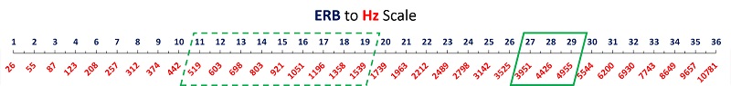
Figure 5.  A ruler showing the relationship between frequency as measured on a psychophysical scale (equivalent rectangular bandwidth, ERB) and a linear Hz scale.  The logarithmic spacing of cochlear filters is illustrated by the green boxes: in the high frequencies, a 1000 Hz range spans 3 normal auditory filters, but in the low frequencies, this same range spans 9 normal auditory filters.  This relationship explains the apparent contradiction by some manufacturers who advertise that their frequency lowering techniques use only a minimal amount of frequency compression.

10. If I understand correctly what you just told me about Speech Rescue, the different sub-regions from the source overlap in frequency after lowering.  Therefore, what difference does the cochlear scaling make if the relationship between the source frequencies is lost after lowering?

Indeed, all of the frequency lowering methods, especially this one, challenge our notions about the nature of high frequency speech information.  We know that most of the speech information transmitted in the high frequencies is in the form of frication (the noisy turbulence produced by the narrowing of the structures in the oral cavity).  We also know that local and global spectral relationships between phonemes in the fricative class (e.g., peak frequency, center of gravity, spectral shape such as flat, sloping upwards/downwards, etc.) bandwidth, and others) and the speech sounds that precede and follow them play an important role in speech perception (e.g., Kent & Read, 2002).  However, we do not have a good knowledge base for how individuals interpret frequency-shifted cues or for what is the best way to transmit them.  Obviously, many of the local (frequency specific) spectral cues are distorted after any frequency lowering of any kind.  At this point, it is an open-ended question as to how frequency lowering can provide benefit.

One under-appreciated source of information for frequency-lowered frication is the temporal envelope.  If you think about it, hearing a fricative shifted down in frequency compared to ‘hearing’ silence, can give you: 1.) information that a speech sound occurred; 2.) information about the sound’s speech class (the fricative sound class); 3.) information about the duration of the frication; 4.) information about the relative intensity of the frication; and, 5.) information about how the intensity changes over time (that is, the temporal envelope, per se).  To highlight the role that this information can play in speech perception, consider that cochlear implants only provide temporal envelope information with gross spectral resolution and that children wearing a cochlear implant have been shown to have better production (and by implication, reception) of the high frequency fricative /s/ compared to children wearing hearing aids (Grant, Bow, Paatsch, & Blamey, 2002).

To illustrate this point in the context of Oticon’s Speech Rescue, Figure 6 shows how the time waveform of a sentence containing several fricatives (Waveform A) is affected by conventional amplification followed by low-pass filtering to simulate a severe to profound high frequency hearing loss (Waveform C) and how this is subsequently affected by Speech Rescue processing (Waveform C).  Now, back to your original question.  Besides having better frequency resolution, one potential advantage to having a greater number of auditory filters to code the lowered signal is a better representation of temporal information across the summed output.  Future research, including cochlear/neural modeling, will help confirm this speculation.

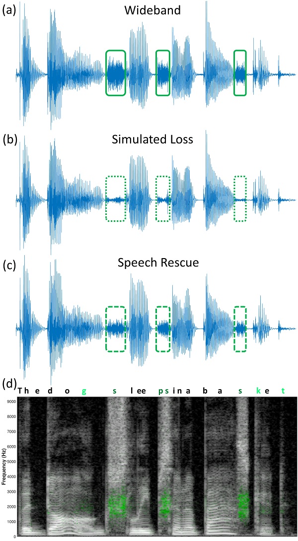
Figure 6.  Plots showing how frequency lowering can contribute to temporal envelope information, using Oticon’s Speech Rescue by way of example.  Waveform A (top) is a time waveform of the sentence “The dog sleeps in a basket” (see text in Waveform D for the correspondence between the waveform and sentence) in quiet as spoken by a male talker from the Hearing-in-Noise Test (HINT).  Here, and throughout, the boxes highlight the phoneme /s/, which is the strongest feature lowered by Speech Rescue in this example.  Waveform B (second from top) is a time waveform of the same sentence but low-pass filtered at 2500 Hz to simulate a complete loss of audibility associated with a severe to profound hearing loss, for example.  Notice an almost complete loss of temporal cues associated with the /s/.  Waveform C (third from top) shows the same sentence in Waveform A, but with Speech Rescue (Configuration 1) applied before low-pass filtering using the same filter that was used to generate Waveform B.  Notice that a good portion of the temporal envelope information from the wideband signal is reintroduced.  Waveform D (bottom) is a comparative spectrogram showing the addition of low-frequency energy around 2000 Hz (green) associated in the action of the Speech Rescue algorithm (compare the frequencies of the green pixels with the destination region shown in the left image in Figure 4 for the same configuration).  Not only can additional low frequency energy be seen for /s/ (letters in dark green in the text), but a little can be seen for the stops /g/, /p/, /k/, and /t/ (letters in light green in the text).  Finally, notice that Speech Rescue retains the original signal in the high frequency spectrum, unlike some other frequency lowering methods.

11. We have yet to talk about frequency compression.  That label seems to be used to describe half of the manufacturers’ products – are they all the same?

They are similar only in some respects.  First, they all work by reducing or ‘squeezing’ the frequency spacing, hence bandwidth, between two limits in the source region.  The lower frequency limit is labeled with different terms, including ‘start frequency,’ ‘f_min,’ and ‘cutoff frequency.’  As shown in Figure 7, frequencies below the start frequency are not subjected to lowering, thereby creating what is known as a ‘broken-stick’ function when plotting output frequency as a function of input frequency.  It can be roughly described by two lines with different slopes, with the lower line having a slope of one.  The start frequency, then, is the frequency where the slope changes.  This feature causes many to classify these techniques as nonlinear frequency compression, which also differentiates it from the full bandwidth frequency compression implemented in AVR Sonovation’s hearing aids (see Alexander 2013b for a more complete discussion of the term nonlinear frequency compression).  The advantage of this method of frequency compression is that the hearing aid can treat one part of the spectrum (the mid to high frequencies) without affecting the other part of the spectrum (the low frequencies).

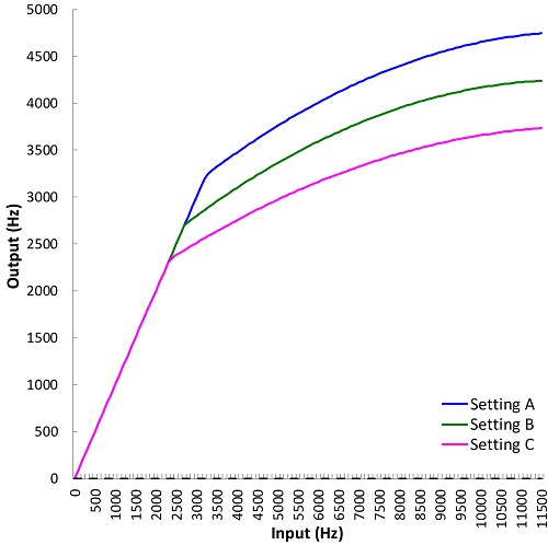
Figure 7.  Plot showing how the frequencies at the input of the hearing aid are altered by nonlinear frequency compression for three different settings (different colors) of Signia’s Frequency Compression (FCo) feature.  Frequencies up to the start frequency (f_min or cutoff) are not altered by algorithms that fall in this class.  Above this frequency, frequencies are compressed and the slope is increased.  On a log-frequency scale, this figure would appear to consist of lines with two slopes (compare with Figure 9, where compression is proportional on a linear scale).  Source: Frequency Compression Fitting Assistant.

In the early devices with this type of frequency lowering, the upper frequency limit in the source region, called ‘f_max’ or ‘maximum output frequency,’ was a fixed distance from the lower frequency limit. That is, the width of the source region was mostly constant.  Now, the upper frequency limit is presumably set by the limits of the microphone and/or analog-to-digital converter that follows.  Both Phonak and Signia have upper frequency limits around 11 kHz, while ReSound has them around 7.3 kHz.  The output frequency that corresponds to the upper limit is determined by the compression ratio, which controls the amount by which the bandwidth of the source region is reduced, or compressed, in the destination region.  Higher compression ratios correspond to more compression and a lower upper-frequency limit (amplified bandwidth).  For audiometric configurations with a more restrictive range of audibility, data that I have collected (Alexander, 2016a) indicates that it is not a good idea to choose aggressive frequency compression settings (lower start frequencies and/or higher compression ratios) in order make a 10 kHz upper limit audible after lowering.  For these cases, I favor less aggressive settings in order to help preserve the speech information in the low frequencies (through the selection of higher start frequencies) and to help preserve the usefulness of the information being lowering (through the selection of lower compression ratios).

12. If I have previously fit patients with frequency compression using hearing aids from one manufacturer, and wish to switch them to another manufacturer when they come in for new hearing aids, can I simply use the same settings?

No!  While the start frequency (or whatever term is used) can be thought of as roughly equivalent across manufacturers, the same cannot be said about the compression ratio.  This is because the frequency compression methods differ in the exact relationship between input and output frequencies and they all use this term to mean different things.  As discussed previously (Alexander, 2013b), the relationship between input and output frequency with Phonak’s SoundRecover was logarithmic.  Furthermore, because the representation of frequency on the cochlea is also logarithmic, the compression ratios could be conveniently mapped onto a psychophysical frequency scale like the ERB scale.  Therefore, a compression ratio of 2:1 meant that an input signal that normally spanned two auditory filters spanned only one auditory filter in the output.

In contrast, with ReSound’s Sound Shaper, the relationship between input and output frequency can be thought of as proportional or linear because the remapping of frequency above the start frequency can be modeled using a simple linear equation (see Alexander 2013b for a detailed discussion about the nuances associated with different equations for frequency compression).  In other words, it is a frequency divider, meaning that for a 2:1 compression ratio, a frequency that is 3000 Hz above the start frequency before lowering will be only 1500 Hz above it after lowering, and so on.  Incidentally, this was exactly the frequency relationship with AVR Sonovation’s technology, which differed in that it always used a start frequency of 0 Hz.  With Signia’s Frequency Compression, about all I can say is that the relationship between input and output frequency cannot be so easily expressed and that it is somewhere between the other two methods.

13. Wow, there sure is a lot to know about frequency lowering!  Now, I am anxious to know what you mean by ‘compression (adaptive)’ in reference to Phonak’s new SoundRecover2 algorithm?

A lot has changed between the original SoundRecover algorithm and the new SoundRecover2 algorithm.  About the only thing that has not changed is that nonlinear frequency compression occurs above a given start frequency.  However, the exact nature of this frequency relationship is adaptive because it varies across time in a way that depends on the spectral content of the source at a given instant.  Specifically, when the source signal has a dominance of low frequency energy relative to high frequency energy, frequency compression is carried out as it was before (Rehmann, Jha, & Baumann, 2016; Glista, Hawkins, Scollie, Wolfe, et al., 2016).  When the source signal has a dominance of high frequency energy, then the frequency-compressed signal undergoes a second transformation in the form of a linear shift or transposition down in frequency.  The original, higher, start frequency (used for low frequency dominated sounds) is called the upper cutoff and the new, lower, start frequency after transposition (used for high-frequency dominated sounds) is called the lower cutoff.  The other major parameter that varies across settings is the maximum output frequency, which designates the output frequency corresponding to the upper frequency limit (a little below 11 kHz).  That is, it determines the amplified bandwidth.  These parameters and their effects on the input-output frequency relationship are shown in Figure 8.

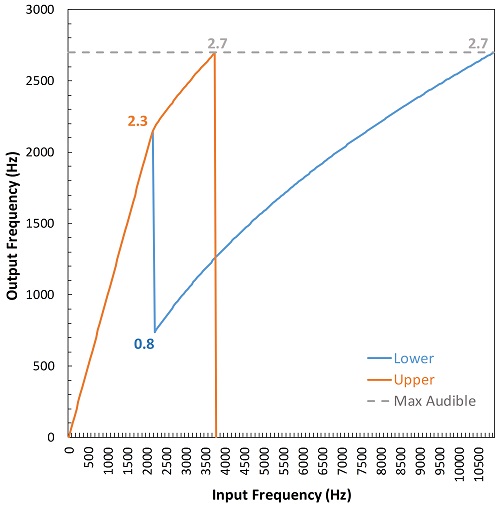
Figure 8.  Plot showing the frequency input-output function for a setting in Phonak’s SoundRecover2.  The orange line shows the function that is activated for low-frequency dominated sounds, which is associated with the upper-cutoff frequency (cutoff2 = 2.3 kHz, in this example).  The blue line shows the function that is activated for high-frequency dominated sounds, which is associated with the lower-cutoff frequency (cutoff1 = 0.8 kHz, in this example).  For both functions, the frequency relationship is linear (no frequency compression) up to the upper-cutoff frequency and is nonlinear up to the maximum output frequency with SoundRecover2 on (2.7 kHz, in this example; which is also shown to be equal to the maximum audible frequency with SoundRecover2 off, the gray dotted line).  The difference between the two functions is that the output frequency corresponding to the upper cutoff is transposed down to the lower cutoff for high frequency-dominated sounds so that there is a greater frequency range to place the lowered signal.  Source: SoundRecover2 Fitting Assistant.

14. What is the purpose of having two cutoff frequencies?

As I (Alexander, 2016a) and others (Ellis & Munro, 2013; Parsa, Scollie, Glista, & Seelisch, 2013; Souza, Arehart, Kates, Croghan, & Gehani, 2013) have indicated, low cutoff (start) frequencies with the typical nonlinear frequency compression (e.g., the original SoundRecover) can be detrimental to recognition of vowels and of several consonants, regardless of the compression ratio.  What I consider low are frequencies in the range of the first and second formant frequencies (spectral peaks corresponding to the vocal tract resonances during speech production) because they are so crucial for accurate recognition of vowels and some consonants and for overall subjective sound quality (e.g., Ladefoged & Broadbent, 1957; Pols, van der Kamp, & Plomp, 1969; Klein, Plomp, & Pols, 1970; Sussman, McCaffrey, & Matthews, 1991; Dorman & Loizou, 1996; Bachorowski & Owren, 1999; Hillenbrand & Nearey, 1999; Neel, 2008).  For example, across experiments, Alexander (2016a) found that a 1.6 kHz cutoff was usually detrimental to vowel and consonant recognition, that a 2.2 kHz cutoff was sometimes detrimental, and that 2.8 kHz cutoff or higher was almost never detrimental.  For reasons like this, the cutoff frequency with SoundRecover was originally restricted to be minimally ~1.5 kHz.  Clinically, this limited the applicability of SoundRecover because individuals with steeply sloping hearing losses starting at lower frequencies did not have audibility for the lowered signal or experienced negative side effects associated with a low cutoff frequency and high compression ratio.

Therefore, one rationale for the two cutoff frequencies is to expand audiometric fitting range for SoundRecover2 by allowing the formant frequencies to be processed with little to no frequency shifting.  The clinician can manipulate this aspect of the algorithm by the selection of the upper cutoff, which is, more or less, controlled by the Clarity–Comfort slider (settings “a” through “d”) in the Phonak Target programming software.  The higher the cutoff, the less likely that formant frequencies and other low frequency content will altered.  In fact, the clinician can essentially turn off frequency lowering for these sounds by setting the upper cutoff to be equal to the maximum output frequency (setting “d” on the Clarity–Comfort slider).

If a high cutoff frequency is selected to maintain perception of low-frequency speech sounds, then, depending on the user’s audiometric configuration, it might be so high that the high frequency information necessary for accurate perception of frication, etc. will not be lowered enough to be in the range of aided audibility.  This is where the second (lower) cutoff frequency comes into play.  An obvious solution would be to simply start frequency compression at a lower frequency for these sounds.  However, the problem is that sometimes a high compression ratio is needed in order bring down into the range of audibility the high frequency energy associated with some fricatives, especially /s/.  This is where the transposition part comes into play.  First, by setting the lower limit of the source region to be equal to the upper cutoff and not to the lower cutoff, fewer frequencies need to be compressed.  Second, by allowing the shift in cutoff to go lower in frequency than before (~0.8 kHz with SoundRecover2 vs. ~1.5 kHz with SoundRecover), the destination region can be made larger.  Not only that, recall from our earlier conversation that the cochlear filters are more densely spaced in the low frequencies.  These three facts combined (narrower source region, wider destination region, denser cochlear filter spacing) mean that, on a perceptual scale, the ratio of the number of auditory filters (ERBs) spanned by the source region to the number spanned by the destination region is smaller.  This is why you will notice that the nominal compression ratio shown on the Target programming software is roughly constant for all of the settings (about 1.5:1).

15. So, if I have a patient that I have previously fit with SoundRecover, can I simply use the same settings for SoundRecover2?

Unfortunately, no.  First, as mentioned, while the nominal compression ratios mean conceptually the same thing, the underlying equations responsible for generating the relationship between input and output frequencies are not the same.  Second, while you can ‘turn off’ the frequency compression for low frequency dominated sounds (setting “d” on the Clarity–Comfort slider), you cannot change the adaptive nature of the frequency compression for high frequency dominated sounds.  And before you tell me that you only care about high frequency speech sounds anyway, you have to consider the frequency shift (transposition) I talked about.  In other words, users will not likely have the same perceptual experience going from the original SoundRecover to SoundRecover2.  Maybe when we meet again, I will be able to talk about independent data that indicates which of the two is better.

16. How do I know the optimal settings to choose?  Is there a generic verification method that can be used for all frequency lowering products?

The answer depends on what exactly you are trying optimize.  If you want to optimize speech perception, then the only real way to know the answer is to measure it for your patient for a large number of settings.  Of course, you then run into the same problems hearing aid fitters had a generation or more ago, when the frequency response of a hearing aid used to be fit this way (Mynders, 2003; 2004).  Namely, it is time consuming and unreliable, which is why prescriptive fitting methods developed in the first place.  Just as each prescriptive fitting method assumes that speech perception will be maximized when the goals of that method are met, one can establish reasonable goals for each method of frequency lowering.  It is then a matter of empirical research to establish whether those are reasonable goals in the first place.

All of the manufacturers provide descriptive terms and instructions for how to adjust the different frequency lowering handles in their programming software based on patient feedback on the subjective sound quality, etc.  However, when fitting children, we have to rely solely on acoustic measures.  I have previously provided a set of generic goals and a generic protocol for using probe-microphone measures with frequency lowering hearing aids (Alexander, 2014).  The primary focus of these is to ensure that frequency lowering does not adversely affect the user’s aidable bandwidth, which is also called the maximum audible output frequency (MAOF).  Generally, the MAOF is measured with frequency lowering deactivated and is chosen to correspond to the frequency where the threshold curve crosses with the curve corresponding to the peak of the Speechmap or to a frequency slightly below it, depending on how much audibility there is between this point and the point where threshold crosses the curve corresponding to the long-term average (see also Scollie et al., 2016 for a discussion of the “MAOF range”).  Furthermore, in order to help clinicians get in the ballpark more efficiently, I have developed the online Frequency Lowering Fitting Assistants I mentioned earlier. They are meant to be used in concert with probe-microphone measures. They show the effects that the different handles have on the relationship between input and output frequencies.  Each of the online Frequency Lowering Fitting Assistants has a link to an instruction page or tips section that outlines the goals for each method, so I will only briefly summarize them here.

For Widex’s Audibility Extender and Enhanced Audibility Extender, the basic idea is to choose the setting that provides complete coverage of the source region after lowering, with the minimum amount of frequency overlap between the un-transposed and transposed signals (see Figure 5 in Alexander, 2013a).  Sticking with transposition-like methods, the goal for Oticon’s Speech Rescue is to choose the lowest configuration for which at least 95% of the destination region is below the user’s MAOF (see Table in Figure 3c in Angelo et al., 2016).

With nonlinear frequency compression methods, it should be obvious that, at minimum, the start frequency (or equivalent term) should be audible in order for the user to hear any of the lowered information.  ReSound’s Sound Shaper only has three settings (Figure 9), so the one that does not restrict user’s aidable bandwidth, if there is one, is the one to choose.  With Signia’s Frequency Compression, the clinician has the option to choose the output frequency corresponding to the upper-frequency limit of the source region, f_max; so, this setting should be equal or greater than the MAOF if the aided bandwidth is to be fully utilized.  As mentioned earlier, the upper limit is ~11 kHz; therefore, one might consider putting f_max slightly higher than the MAOF, which will trade the amount of high frequency information that is audible after lowering for a more favorable (lower) compression ratio.  At the other end, I already talked about the advantages of keeping the start frequency, or f_min, high.  However, it should not be so high that the audible destination region becomes restricted to point where the information contained therein is useless because of a high compression ratio.  Similar concepts were embraced with my fitting assistants for the original SoundRecover, which took the start frequency, compression ratio, and the user’s aided bandwidth all into consideration.  However, with SoundRecover2, a different approach has to be taken.

Figure 9.  Plot showing the frequency input-output functions for the three settings available in ReSound’s Sound Shaper (different colors).  Notice that compared to Figure 6, these lines have the appearance of ‘broken-stick’ functions (two lines, with different slopes) on a linear frequency scale.  This is a byproduct of the ‘proportional’ compression discussed in the text. Source: Sound Shaper Fitting Assistant.

17. How is SoundRecover2 different?

For one, the adaptive nature of the algorithm means that the start or cutoff frequency can be different for the low and high frequency dominated speech sounds, so some of the negative side effects we talked about earlier are less of a concern.  For another, because some settings have the same “maximum output frequency” (output frequency of the upper frequency limit in the source region), similar to the scenario for Signia’s f_max, goals cannot be determined solely on its placement either.

While there are more variables at play with SoundRecover2 than with any other method, Phonak has kept it easy for the clinician by constraining the number of options in their programming software.  First, let’s start with the Audibility-Distinction slider.  It has 20 different options that vary according to the audiogram entered into the software.  Moving this slider from left to right (from Audibility to Distinction or 1 to 20) progressively increases the lower cutoff and the maximum output frequency.  Given that we do not want to adversely reduce the aided bandwidth, only those settings where the maximum output frequency is equal to greater than the MAOF should be considered.  Furthermore, as we discussed with Signia’s f_max, putting it slightly higher is probably OK, or even desirable, since we probably do not need to make all of the information up to 11 kHz audible after lowering in order to maximize speech perception.  After this is set, the clinician must choose from one of four settings (a to d) on the Clarity-Comfort slider.  The main change associated with this slider is the upper cutoff, which not only controls how low-frequency dominated sounds are processed, but also changes the lower limit of the source region for high frequency dominated sounds.  As mentioned, setting “d” essentially turns off the frequency lowering for the former since the upper limit is equal to the maximum output frequency.

Now that we have reduced the 80 possible combinations of settings to a reasonably small set, which one should you choose?

18. I don’t know, how should we choose the optimal setting?

Sorry, I only was posing a rhetorical question.  Remember, optimization is relative to our pre-established goals.  In this case, because of the variable effects on the acoustics, I'll answer this question in the context of the speech sounds that we wish to enhance with frequency lowering, namely high frequency fricatives like /s/.  While we can find several settings that make the /s/ audible after lowering, it was recognized long ago (e.g., Simpson, 2009; Kuk, Keenan, Korhonen, & Lau, 2009; Auriemmo et al., 2009; Wolfe et al., 2011; Alexander, 2015) that one of the biggest problems with lowering the /s/ is that it becomes confused with the /ʃ/, which has similar properties but a lower spectral center of gravity, which is related to the spectral peak.

For as long as they have been talking about frequency lowering, Susan Scollie and her colleagues at Western University have advocated for selecting settings that acoustically increase the /s/-/ʃ/ distinction on probe-microphone measurements (e.g., Glista & Scollie, 2009; Scollie, 2013; Mueller et al., 2013; Glista, Hawkins, & Scollie, 2016; Scollie et al., 2016).  They have gone to the effort to create calibrated versions of these sounds for use on probe-microphone systems.  With the original SoundRecover, and other methods of frequency lowering, clinicians were to use these signals to see where the upper frequency shoulders of their spectra overlapped.  However, upon inspection of how SoundRecover2 affected these signals, I noticed that the selection of the lower and upper cutoffs, especially the upper cutoff (remember, this is mainly controlled by the Clarity-Comfort slider after the other slider has been set), also affected the amount of overlap along the lower-frequency shoulder of the spectra.  This primarily occurs because the spectral content of these signals is processed without frequency compression up to the upper cutoff and is then abruptly shifted down in frequency due to the transposition we talked about earlier.  Because the spectrum for /ʃ/ spreads to relatively low frequencies, this means that its lower-shoulder frequency does not shift as the upper cutoff is raised above a certain point while it continues to increase for /s/.  Therefore, this opens up the opportunity to increase the acoustic distinction and, perhaps, enhance the perceptual distinction between this pair of sounds by manipulating the lower-shoulder frequency.  This may be particularly important for those settings on the Audibility-Distinction slider that generate identical upper-shoulder frequencies for the lowered /s/ and /ʃ/.

19. Can you please provide some visuals to help me understand these difficult concepts?

Figure 11 illustrates some of these points, but let me briefly describe how I have incorporated them into my fitting assistant for SoundRecover2.  To use it, enter the MAOF (in Hz to correspond to the units shown on most probe-microphone systems), the lower and upper cutoffs (in kHz, as reported by the Phonak Target programming software as cutoff1 and cutoff2, respectively), and the maximum output frequency.  The values for the settings can be found by hovering the mouse over the graphical display in the Phonak Target programming software that shows the estimated frequency response of the output.  Besides, showing the usual relationship between input and output frequencies as estimated from acoustic measurements and from the values shown in the programming software, I also show how /s/ and /ʃ/ are affected by the different settings.  Using the signals available from Western University, I computed the 6 dB down points for the /s/ and /ʃ/ to roughly approximate the lower and upper-shoulder frequencies and to what I could visually observe on the Audioscan Verifit before and after lowering.  The input/output ranges for /s/ are plotted using green lines since this signal shows up first on the alphabetically arranged list and because green is used to color the first Speechmap conducted on the Audioscan Verifit.  Likewise, /ʃ/ is plotted in purple and magenta colors.  The thicker line for each signal corresponds to the logarithmic center (on an ERB scale) of the two shoulder frequencies.  Remember, what I said about ‘optimizing’ relative to a concrete goal?  If our goal is to maximize the spectral distinction between /s/ and /ʃ/, then we need to consider both the lower and upper spectral shoulders.  To help the clinician with this judgment, the fitting assistant estimates the number of auditory filters (ERBs) that are non-overlapping on both sides of the spectra.

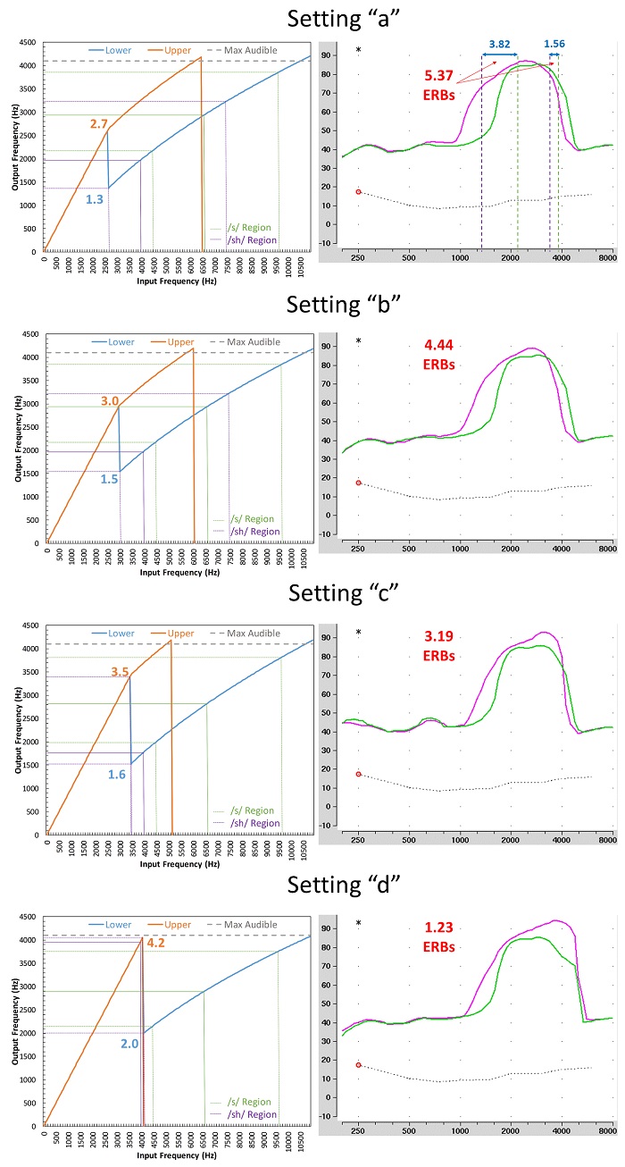
Figure 10.  Plots showing how the settings for the Clarity-Comfort slider (settings “a” to “d”) for a fixed setting on the Audibility-Distinction slider affect the frequency input-output relationship (left column) and the spectra as measured by the Audioscan Verifit (right column) for the Western University /s/ (green line) and /ʃ/ (magenta line).  The maximum output frequency with SoundRecover2 activated (set by the Target programming software) was 4.2 kHz and the values for the lower and upper cutoffs (cutoff1 and cutoff2, respectively) are shown on the frequency input-output functions in blue and orange text respectively.  As shown, as one goes from setting “a” to setting “d”, the primary effect is on the value for the upper cutoff, which also determines the lower frequency limit of the source region for the lower cutoff (see Figure 7 and associated descriptions).  As shown by the dotted lines for each plot in the left column, the SoundRecover2 Fitting Assistant estimates the lower- and upper-shoulder frequencies of the /s/ (green) and /ʃ/ (purple) after frequency lowering.  It then computes the absolute cochlear-scaled difference in ERB-units between both the upper and the lower shoulders of the two spectra (see spectra for setting “a”).  Presumably, but not definitively, the setting that maximizes the representation of the /s/ and /ʃ/ on the cochlea will be the most discriminable for this pair of sounds, and perhaps for other pairs.  Keep in mind that the Audioscan Verifit analyzes the frequency response using 1/3-octave wide filters every 1/12 octave, so for some settings, the values shown on the fitting assistant and those shown on the Speechmap may appear to differ by a few hundred Hz.  Specifically, the spectral rolloff of /s/ and /ʃ/ may appear to be more gradual that what it actually is and/or the bandwidth may appear to be slightly wider (see the marked up example for setting “a”).

It is important to note a few things about verification and validation.  The online Frequency Lowering Fitting Assistants are not intended to substitute for what the clinician observes with actual electroacoustic measurements, but they should be close and should help objectify the process of deciding which settings to evaluate with the user.  For a detailed step-by-step protocol to verify fittings with frequency lowering, see An Update on Modified Verification Approaches for Frequency Lowering Devices by Glista, Hawkins, & Scollie (2016). The clinician will want to use probe-microphone measurements to ensure that the lowered speech is audible, and depending on the frequency lowering method, to confirm spectral differences between /s/ and /ʃ/.  Post-fitting outcome measures, in addition to user or parent report, may include speech testing such as plural (/s/ and /z/) detection (e.g., the UWO Plurals test) and discrimination words with /s/ and /ʃ/ as minimal pairs.

In order to simplify the process of fitting a patient with frequency lowering on a Monday morning, here is a generic protocol that will work fairly well with most of the methods we have discussed (see also, Alexander, 2014):

1. Deactivate the frequency lowering feature and fit the hearing aid to prescriptive targets using probe-microphone measures as you would normally do for a conventional hearing aid.
   1. Find the maximum audible output frequency, MAOF, which is the highest frequency in the real-ear aided output that exceeds threshold on the SPL-o-gram (Speechmap).  This point can be defined somewhere between the average and peaks of the amplified speech range; the exact point is subject to debate so consistency between measures is most important.
   2. Enter the MAOF in the online Frequency Lowering Fitting Assistant for the frequency lowering method you are using in Hz to match the units displayed by most hearing aid analyzers.
2. Activate the frequency lowering feature and use the fitting assistant to position the lowered speech within the audible bandwidth (MAOF) while not reducing it further.
   1. Most of the destination region should be audible.
   2. Avoid too much lowering, which will unnecessarily restrict the bandwidth you had to start with and may reduce intelligibility.
3. With the chosen settings activated, verify that the MAOF is reasonably close to what it was when it was deactivated in Step 1.  Sometimes it may be slightly higher, which is OK.  If it is unacceptably lower, try increasing gain in the channels near the MAOF.  Rarely, a weaker setting will have to be chosen in order to maintain the audible bandwidth.  If a better estimate of the maximum audible input frequency is desired, the value for MAOF from this step should be entered into the fitting assistant.

One more thing.  Notice that for the probe-microphone measures, we are using the specially designed signals from Western University as the input signal.  Many clinicians, however, have become accustomed to using the Audioscan Verifit 1/3-octave filtered speech to quantify aided audibility of the lowered signal.  I can recommend these, perhaps, but only for verifying audibility of speech lowered by Widex’s Audibility Extender and Enhanced Audibility Extender.  For the others, a problem arises because the bandwidth of these signals is narrower than the actual speech signals that occupy these bands.  Therefore, the levels of these signals will not reflect what will happen with full bandwidth speech.

Take the frequency compression algorithms, for example.  In these cases, because the 1/3-octave input band is subjected to frequency compression, the bandwidth of the output for this region is less and is inversely proportional to the compression ratio.  Therefore, the level measured by the 1/3-octave analysis bands may be lower than what it would be for the full-spectrum speech signal.  Not only is it not a valid indicator of audibility, my own experiences indicate that it is not reliable, since the magnitude of the effect seems to depend on a complex interaction between the architecture of the filter bank in the hearing aid and the center frequency of the analysis band closest to the peak of the lowered signal. 

(a)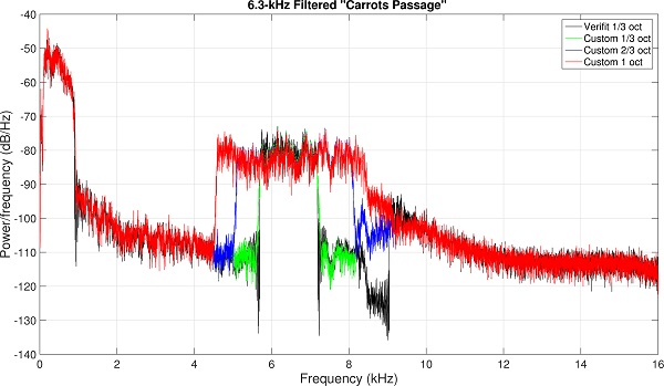  

(b)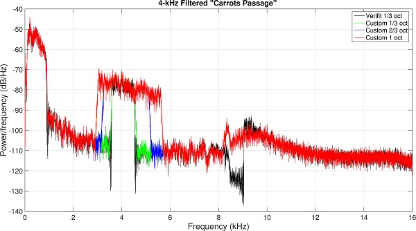 

Figure 11.  Spectra of the ‘special’ speech signals centered at 6.3 (top) and 4.0 kHz (bottom) that were used to evaluate hearing aid output in response to frequency compression shown in Figure 12.  Black shows the spectra of the 1/3-octave wide test signals provided by the Audioscan Verifit, green shows the spectra of the matching 1/3-octave wide test signals I created, blue shows the spectra of my custom 2/3-octave wide test signals, and red shows the spectra of my custom 1-octave wide test signals. 

To illustrate the limitations of using a 1/3-octave filtered speech band to assess audibility, a series of measurements using the Audioscan Verifit and a Phonak Bolero Q90-SP hearing aid were conducted.  First, using the full spectrum “carrots passage” from Audioscan, the filtering used to create the 1/3-octave filtered speech centered at 6.3 kHz (Figure 10a) and at 4.0 kHz (Figure 10b) was replicated.  The spectrum of the Audioscan Verifit signal is in black and the spectrum of the custom, matched signal is in green.  Using these techniques, the bandwidth of the filtered speech was extended to 2/3 octave (blue) and to 1 octave (red).  I then used the Audioscan Verifit to present them to the Bolero hearing aids.  The first setting (Figure 11a) was programmed to a 20-dB HL flat audiometric profile and the linear gain option was selected in the Target programming software. SoundRecover was set to a 1.5-kHz start frequency and a 2.8:1 compression ratio (in theory, because frequency compression is linear on a log scale, this would be a 2.8 times reduction in the bandwidth of the filtered speech).  As can be seen, at the 3000-Hz analysis band, the level of the 6.3-kHz 1/3-octave filtered speech (magenta line) is significantly below the level of the full-spectrum speech signal (green line).  In contrast, the 2/3-octave (blue line) and 1-octave (orange line) filtered signals are essentially equivalent to the full-spectrum speech signal at this frequency.  The second setting (Figure 11b) was programmed to a 60-dB HL flat audiometric profile and the nonlinear gain option was selected.  SoundRecover was set to a 1.5-kHz start frequency and a 4.0:1 compression ratio.  Again, there seems to be no difference between the 2/3-octave and 1-octave filtered speech (4-kHz center frequency), both of which had higher levels at the 2000-Hz analysis band than the 1/3-octave filtered speech.

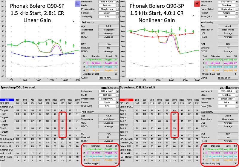
Figure 12.  Audioscan Verifit Speechmap for the standard speech passage and the test signals shown Figure 11 (6.3 kHz signal left image; 4.0 kHz signal, right image).  See text for details about how each hearing aid was programmed.  The tables show how the output at the 1/3-octave wide analysis bands at the frequencies closest to the location of the lowered signal (3000 Hz for left image, and 2000 Hz for right image) are affected by the bandwidth of the test signals.  For both hearing aid settings, the level of the 1/3-octave filtered speech (Test 2, magenta line) is significantly below the level of the full-spectrum speech signal (Test 1, green line).  In contrast, the 2/3-octave (Test 3, blue line) and 1-octave (Test 4, orange line) filtered signals are essentially equivalent to the full-spectrum speech signal at this frequency.

20.  So, the past ten years have been quite the ride for frequency lowering.  What do you see happening with this technology in the next decade?

I think that as limitations in processing time are reduced with faster and more efficient chips, and as limitations in current drain are reduced with rechargeable batteries, that hearing aid algorithms in general will become more selective in how they operate.  We have already seen this starting to happen with more tried-and-true algorithms like amplitude compression, noise reduction, and directionality.  Depending on the acoustics and the hearing aid’s assessment of the listening situation, these algorithms not only activate and deactivate selectively, they can also vary the ‘aggressiveness’ of their parameters to anticipate the user’s needs and preferences.

Specifically, with regard to frequency lowering, one of the primary findings from Alexander (2016a), which examined vowel and consonant identification across a half dozen different nonlinear frequency compression settings, was that no one set of parameters simultaneously maximized recognition for all tokens.  That is, the parameters that lead to the highest identification rates for individual consonants seemed to vary according to their acoustic characteristics as determined by the individual talker and the vowel context.  Settings that maximized the identification of one consonant sometimes came at the expense of a decrease in the identification of one or more consonants.  With more knowledge about when and how to implement each specific type of frequency lowering method and with signal processing constraints lessened, it is not hard to imagine a smart hearing aid that fine tunes frequency lowering parameters on the fly to accommodate differences between talkers and phonetic context.  Regardless if I am right or wrong, the next ten years promises to be a very exciting time in hearing aid technology!

References

Alexander J.M. (2013a).  Individual variability in recognition of frequency-lowered speech.  Seminars in Hearing, 34, 86-109.

Alexander, J.M. (2013b).  20Q: The Highs and lows of frequency lowering amplification. AudiologyOnline, Article #11772.  Retrieved from www.audiologyonline.com

Alexander, J.M. (2014).  How to use probe microphone measures with frequency-lowering hearing aids. Audiol Prac, 6(4), 8-13.

Alexander, J.M. (2015).  Enhancing perception of frequency-lowered speech -   Patent No. US 9,173,041 B2. Washington DC: US Patent and Trademark Office.

Alexander, J.M. (2016a).  Nonlinear frequency compression: Influence of start frequency and input bandwidth on consonant and vowel recognition. J Acoust Soc Am, 139, 938-957.

Alexander, J.M. (2016b).  Hearing aid delay and current drain in modern digital devices. Canadian Audiologist, 3(4).

Angelo, K., Alexander, J.M., Christiansen, T.U., Simonsen, C.S., & Jespersgaard, C. F.C. (2015).  Oticon frequency lowering: Access to high-frequency speech sounds with SpeechRescue technology. Oticon white paper, retrieved from: https://www.oticon.com/~/media/Oticon US/main/Download Center/White Papers/43698 Speech Rescue White Paper 2015.pdf

Auriemmo, J., Kuk, F., Lau, C., Marshall, S., Thiele, N., Pikora, M.,…Stenger, P.  (2009).  Effect of linear frequency transposition on speech recognition and production of school-age children. J Am Acad Audiol, 20, 289-305.

Bachorowski, J., & Owren, M. (1999).  Acoustic correlates of talker sex and individual talker identity are present in a short vowel segment produced in running speech. J Acoust Soc Am, 106, 1054-1063.

Dorman, M.F., & Loizou, P.C. (1996).  Relative spectral change and formant transitions as cues to labial and alveolar place of articulation. J Acoust Soc Am, 100, 3825-3830.

Ellis, R., & Munro, K. (2013).  Does cognitive function predict frequency compressed speech recognition in listeners with normal hearing and normal cognition? Int J Audiol, 52, 14-22.

Galster, J.A.  (2015).  The prescription of Spectral IQ.  Starkey technical paper, retrieved from: https://starkeypro.com/pdfs/technical-papers/The_Prescription_Of_Spectral_iQ.pdf.

Glasberg B.R., & Moore B.C.J. (1990).  Derivation of auditory filter shapes from notched-noise data.  Hear Res, 47, 103-138.

Glista, D., & Scollie, S. (2009).  Modified verification approaches for frequency lowering devices. AudiologyOnline, Article #2301. Retrieved from www.audiologyonline.com

Glista, D., Hawkins, M., & Scollie, S. (2016).  An update on modified verification approaches for frequency lowering devices. AudiologyOnline, Article #27703.  Retrieved from www.audiologyonline.com

Glista, D., Hawkins, M., Scollie, S., Wolfe, J., Bohnert, A., & Rehmann, J. (2016).  Pediatric verification for SoundRecover2. Best practice protocol.  Available from Phonak AG.  Retrieved from www.phonakpro.com/content/dam/phonakpro/gc_hq/en/products_solutions/pediatrics/documents/best_practice_protocols/best_practice_protocol_sound_recover2_pediatric_verification.pdf

Grant, L., Bow C., Paatsch, L., & Blamey, P. (2002, December).  Comparison of production of /s/ and /z/ between children using cochlear implants and children using hearing aids. Poster presented at: Ninth Australian International Conference on Speech Science and Technology, Melbourne Australia.

Hillenbrand, J., & Nearey, T. (1999). Identification of resynthesized /hVd/ utterances: Effects of formant contour. J Acoust Soc Am, 105, 3509-3523.

Jongman, A., Wayland, R., & Wong, S. (2000).  Acoustic characteristics of English fricatives. J Acoust Soc Am, 108, 1252-1263.

Kent, R.D., & Read, C. (2002).  Acoustic analysis of speech, 2^nd edition (Thomson Learning: Canada).

Klein, W., Plomp, R., & Pols, L.C.W. (1970).  Vowel spectra, vowel spaces, and vowel identification. J Acoust Soc Am, 48, 999-1009.

Kuk, F., Keenan, D., Korhonen, P., & Lau, C. (2009).  Efficacy of linear frequency transposition on consonant identification in quiet and in noise. J Am Acad Audiol, 20, 465-479.

Kuk, F., Schmidt, E., Jessen, A. H., & Sonne, M. (2015).  New technology for effortless hearing: A “Unique” perspective. Hearing Review, 22(11), 32-36.

Ladefoged, P., & Broadbent, D. E. (1957).  Information conveyed by vowels. J Acoust Soc Am, 29, 98-104.

Mueller, H.G., Alexander, J.M., & Scollie, S. (2013).  20Q: Frequency lowering - the whole shebang. AudiologyOnline, Article #11913.  Retrieved from www.audiologyonline.com

Mynders, J.M. (2003).  Essentials of hearing aid selection, Part 2: It’s in the numbers. Hearing Review, 10(11).

Mynders, J.M. (2004).  Essentials of hearing aid selection, Part 3: Perception is reality. Hearing Review, 11(2).

Neel, A. (2008).  Vowel space characteristics and vowel identification accuracy. J Speech Lang Hear Res, 51, 574-585.

Parsa, V., Scollie, S., Glista, D., & Seelisch, A. (2013).  Nonlinear frequency compression: effects on sound quality ratings of speech and music. Trends in Amplification, 17, 54-68.

Pols, L.C.W., van der Kamp, L.J.T., & Plomp, R. (1969).  Perceptual and physical space of vowel sounds. J Acoust Soc Am, 46, 458-467.

Rehmann, J., Jha, S., & Baumann, S.A. (2016).  SoundRecover2 – the adaptive frequency compression algorithm: More audibility of high frequency sounds. Available from Phonak AG.

Scollie, S. (2013).  20Q: The ins and outs of frequency lowering amplification. AudiologyOnline, Article #11863. Retrieved from www.audiologyonline.com

Scollie, S., Glista, D., Seto, J., Dunn, A., Schuett, B., Hawkins, M.,…Parsa, V. (2016).  Fitting frequency-lowering signal processing applying the American Academy of Audiology Pediatric Amplification Guideline: Updates and protocols.  J Am Acad Audiol, 27, 219-236.

Simpson, A. (2009).  Frequency-lowering devices for managing high-frequency hearing loss: A review.  Trends in Amplification, 13, 87-106.

Souza, P.E., Arehart, K., Kates, J., Croghan, N.E., & Gehani, N. (2013).  Exploring the limits of frequency lowering. J Speech Lang Hear Res, 56, 1349-1363.

Sussman, H., McCaffrey, H.A., & Matthews, S.A. (1991).  An investigation of locus equations as a source of relational invariance for stop place categorization. J Acoust Soc Am, 90, 1309-1325.

Wolfe, J., John, A., Schafer, E., Nyffeler, M., Boretzki, M., Caraway, T., & Hudson, M. (2011). Long-term effects of non-linear frequency compression for children with moderate hearing loss. Int J Aud, 50, 396-404.