
Editor’s Note: This text course is an edited transcript of a live seminar on AudiologyOnline, presented in partnership with Siemens Hearing Instruments, Inc. Download supplemental course materials here.
Dr. Harvey Dillon: It is a pleasure to be talking to you all, especially without the 20-hour flight to get from Australia to the U.S. Let’s get right into our topic, the NAL-NL2 prescription.
Before getting into the intricacies of the prescription, I want to reassure you that using NAL-NL2 is as simple as using any of the previous National Acoustic Laboratories (NAL) prescriptions. For an adult hearing aid fitting, the clinical process won’t change with this new prescription. That process involves measuring hearing thresholds and entering those thresholds into whatever software you are using. Usually the hearing aid manufacturer’s software has the NAL-NL2 algorithm incorporated, and then we verify that with a real-ear measurement and adjust the amplification to match the prescription.
For children, we recommend a variation to the procedure where the thresholds are measured or estimated on the basis of electrophysiology. Individual real-ear-to-coupler differences (RECD) are either measured or estimated on the basis of age. Those two sets of information are entered into the manufacturer’s software; or alternatively into standalone software incorporating NAL-NL2, also. The result of that is a coupler prescription, to which a hearing aid is adjusted to match. The real-ear effects have already been taken into account via the RECD.
The goals of the NAL-NL2 are to make speech as intelligible as possible and to make loudness comfortable. We know very well that people want additional things from their hearing aids - such as localization, a nice tonal quality, the ability to detect sounds around them, and sound naturalness – and there are many variables that affect these qualities. The trouble is, we do not really know how to quantify them, and so we focused on intelligibility and loudness, which we suspect may be more important than the other factors.
The main question posed is, “How much amplification?” Hearing aids are very sophisticated, and they make very complex decisions about how much gain to apply when and where. The end result of all of that is amplification at each frequency. That is what the NAL-NL2 prescription is aimed at specifying.
I want to make an analogy with a lolly shop, where a child goes into the lolly shop with an allotted amount of money and wants to come out with the best possible taste experience. The child may have a favorite lolly, but why spend all his money on that one lolly when he can get a broader experience by having a range of sweets? Consider that not all the sweets are equally good, so the child may well spend more of his money on the favorite lolly than on any other lolly. It is the same with gain and frequency response. We have a budget, which in our case is a loudness budget. If we make the hearing aid too loud, people will not like the hearing aid. We have to spend that loudness budget by applying gain at different frequencies with different amounts. We want to spend the budget most wisely, namely concentrating on those frequencies where we can make the biggest contribution to intelligibility.
Developing NAL-NL2
The goal in developing NAL-NL2 was specifically to maximize speech intelligibility, but keep the loudness less than or equal to normal loudness. That is the loudness that would be perceived by a normal hearing person listening to the same sound. NAL-NL1 was actually based on the same goals, but in the decade or more since then, we have had a number of empirical studies, mostly led by Dr. Keidser, which have given us information about how well NAL-NL1 does or does not achieve its aims. Believe me, we know more about the deficiencies in NAL-NL1 than anybody else, and that has provided useful data into guiding the derivation of NAL-NL2. We also had some specially-designed experiments in order to find out more about how much information hearing-impaired people can extract from speech at different levels for different degrees of hearing loss.
Here is how the basic derivation works. Start with a speech spectrum and level. Just pick one. Let us choose 65 dB speech, for instance, and the spectrum that normally goes with it. Assume some arbitrary gain frequency response, and that will then tell us what the amplified speech spectrum is. If we put that into a model for predicting intelligibility, the result is the intelligibility achieved for that particular gain-frequency response. If we then make an iterative adjustment to the gain frequency response, we can keep adjusting it in the direction that increases the predicted intelligibility according to the model. In other words, we have a calculation loop. So we are traveling around this loop, changing the gain each time at each frequency in order to maximize the intelligibility.
You can guess what would happen if this is all we did. We would end up with a lot of gain at all frequencies, and everything would come out sounding loud, no matter what the original speech signal was. Doing that by itself is not enough. We also need to calculate the loudness that is a consequence of each gain-frequency response. That predicts what the loudness would be for the hearing-impaired person.
So how does it compare to the loudness that a normal-hearing person would perceive? To answer this, we also apply the loudness model to the unamplified speech spectrum to predict what the normal loudness would be. We can then compare the normal-hearing loudness to the hearing-impaired loudness. If it is too loud, then we simply turn the gain down at all frequencies.
We have two loops, one where the individual gains and individual frequencies are being turned up or down to maximize intelligibility, and one which is turning the overall gain down so that the overall loudness is equal to, or no more than, normal-hearing loudness. Both loops work simultaneously. Eventually, this process converges on a solution, and what we then have is the predicted gain frequency response for a particular audiogram and for a particular speech input level and spectrum.
We repeated that process for a range of many audiograms. It was meant to cover a wide range of possible audiograms and a wide range of input levels. We end up with a prescribed optimum gain for each of those combinations (Figure 1).
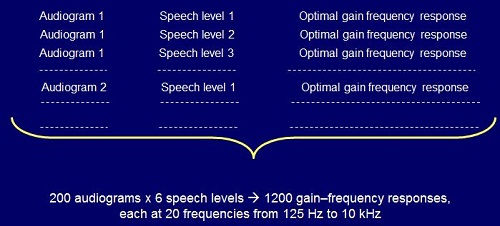
Figure 1. Process for deriving gain frequency responses for NAL-NL2.
That process, of course, is of no use to an individual clinician. That is just the background process that we went through, which produced these set of optimum gain frequency responses. What we then have to do is to bring it into a formula that is easy to implement in software.
That is not all we did. The derivation I have so far described is all very theoretical. The intelligibility model is based on real data from real people, but it is still a theoretical prediction based on psychoacoustics and speech science, along with the assumptions of maximizing intelligibility and controlling loudness. We need to be able to build in the empirical observations that we have collected over the last decade, and even the ones going back before then.
If there is a disagreement, we need to make an adjustment to the assumptions or the rationale so that we do end up with a prescription that agrees with what we have empirically found people prefer and do best with. That is the process we have used here. We will talk more about the adjustments later in this talk.
The result of all that is a final formula. In this case, we have produced the final formula with something called a neural network. A neural network is where you put inputs in. In this case, the inputs were the audiogram values and the overall sound pressure level of speech. We know what the right answers are for our examples, because we chose the audiograms and the sound pressure levels, so we know what gains came out of the optimizer.
Because we have the right answers for many audiograms, each combined with several sound levels, that means we can train the neural network. Training the neural network will then produce the gains for any other audiogram sound pressure level that is within the broad range of those used for training. The end result of our derivation is actually the coefficients of a neural network, which actually just represents a complicated formula. In other words, we end up with a formula that summarizes that derivation process that I have talked about. The two key ingredients of the derivation process are the loudness model and the speech intelligibility model.
The Loudness Model
We have not changed anything in the loudness model. We have entirely adopted the loudness model of Moore and Glasberg (2004). It is a sophisticated model, and we are happy to be able to use it. The intelligibility model is our own variation of the standard speech intelligibility index (SII), also known as articulation index, which I will also talk about.
The basic rationale for predicting intelligibility is based on the speech spectrum. Figure 2 is an illustration, characterized by a 30 dB dynamic range on a graph of 1/3 octave SPL versus frequency. We then compare that to the person’s threshold. Anything above the threshold is audible, and anything below the threshold is not audible. If there is noise present, then we also need to only take into account the parts of the speech spectrum that are above the noise and the threshold. Only the shaded region is audible, so that is the proportion of the information that is coming through (Figure 2). We can quantify that by the number of decibels that are audible at each 1/3 octave frequency.
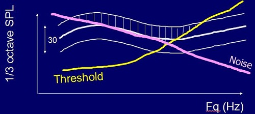
Figure 2. Predicting intelligibility based on audibility (shaded region) above hearing threshold (yellow) and noise (pink).
Of course, not all frequencies are equally important. Just like in a lolly shop, not all the lollies are equally desirable. We know that the very low and the very high frequencies do not contribute as much to intelligibility as the mid frequencies. So what we can do is multiply each of those audibilities times the importance of each frequency, and that gives a contribution to intelligibility of each frequency. These can then be summed. In this particular example (Figure 2), the calculation comes to 0.3, or 30%. Roughly speaking, ignoring the variation of importance with frequency, we can say that about 30% of that speech spectrum is audible to the person in this example. That is the standard SII calculation method, summarized by this formula:
SII = Σ Ai Ii at each frequency, which is characterized by i.
There is a third twist to that, and that is that if you make speech too loud, intelligibility, even for normal hearers, actually goes down because there is more spread of masking in the cochlea. There is a level-distortion factor that is not represented in that formula. Here is how that happens. As the speech level rises above 73 dB, the SII model tells us that the level-distortion factor decreases below 1. In other words, you get smaller contributions to intelligibility the louder you make it.
That is a bit of a problem with hearing-impaired people, because if we do not make it louder, then we do not get audibility. So right in there is the tradeoff that we are making with hearing-impaired people. We want gain for audibility, but not too much gain, or we start to degrade intelligibility, as well as making the sound unnatural to them. If a soft sound is amplified to be something that sounds very loud, then it will sound out of place to people.
So what do we do with that SII number? We can turn that into percent correct using something called the transfer function. Depending on how difficult the speech material is, there are different transfer functions. If we are dealing with sentences, an SII of 0.3, for instance, might give us 80% correct, whereas with nonsense syllables, an SII of 0.3 might only give us 35% correct.
How well does this calculation method work? For people with normal hearing, it works pretty well. For people with mild hearing loss, it also works well. By the time we get to severe hearing loss, it does not work that well.
Ching, Dillon & Byrne (1998) measured speech intelligibility at different sensation levels and predicted intelligibility from the model (Figure 3). For mild flat losses and mild sloping losses, the prediction is reasonably close to the measured data. Once we get into the severe range, the predictions always over-predict the amount of intelligibility listeners will receive. Because of distortions in a damaged cochlea, people with hearing impairment experience reduced frequency selectivity and reduced temporal selectivity. They cannot extract as much information as a normal-hearing person can, even when it is audible.
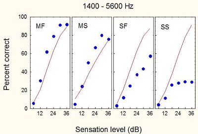
Figure 3. Sensation levels for individuals with mild flat (MF), mild sloping (MS), severe flat (SF) and severe sloping (SS) hearing losses. The blue dots correspond to percent-correct as the sensation level of the stimuli increases.
We experimented with 20 normal-hearing subjects and 55 with a wide range of hearing losses to find out how much information people can extract from speech at different frequencies when amplified by different amounts. We ended up with several measured results and some predicted curves, which I will not go into. There is large scatter, and there are reasons for that, but what we are interested in is how deficient a person is compared with the expected result.
Figure 4 shows the transfer function, the yellow curve showing the relationship between expected percent correct and SII. We can get this transfer function for normal listeners. The expected result for the hearing-impaired population will be worse than the normal-hearing function. The question is, “How much worse?”
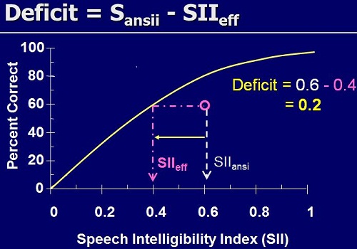
Figure 4. Transfer function indicating the intelligibility deficit faced by listeners with hearing impairment. This example shows that an individual scores 60% correct with an SII of 0.6, whereas a normal-hearing individual would score 60% correct at an SII of 0.4.
Suppose this is a particular result for a particularly hearing-impaired person listening to speech filtered and amplified in a particular way. There is a deficit, because the point is below the line (Figure 4). We can quantify that deficit not by a low percent-correct score, but by how much information it seems like the person is getting. They are getting 60% correct, and a normal-hearing person would get 60% correct with an SII of only 0.4, or with only 40% of the information available. This hearing-impaired person has physically had available 60% of the information, and they also got 60% correct (which is a coincidence). However, there is a deficit in SII of 0.2 that we need to somehow explain on the basis of their hearing loss.
We calculated those deficits using nonsense syllables and sentences. There is a reasonable correlation between the two, so we are measuring something intrinsic about the person’s ability to extract information from speech, whether that speech is nonsense syllables or sentences.
What do we do with that information? We have to somehow modify the SII model to incorporate this reduced ability to extract information. We call this desensitization, which is not a great word, but that is the word that seems to have been adopted.
As you increase the sensation level from 0 to 30 dB, the amount of information extracted from speech goes from 0 to 1 (i.e. 100%) for a person with normal hearing. It appears that hearing-impaired people cannot extract the same amount of information, so we need a different curve that rises to a different maximum that is less than 1. Our data have indicated for low-sensation levels just above 0 that hearing-impaired people are pretty good at extracting information, almost the same as normal hearers. As you go on increasing the sensation level, normal hearers keep on getting more and more information out; whereas, hearing-impaired people are less able to extract more information.
How much less depends on how much hearing loss they have. We fitted a model to our speech intelligibility data that lets us predict this parameter m, which is the maximum information that we could extract, and also the parameter p, which controls how quickly they go from normal to non-normal as the sensation level rises (Figure 5).
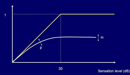
Figure 5. Intelligibility and audibility; the yellow line indicates a normal-hearing person’s ability to understand as sensation level increases; the white line indicates a hearing-impaired person’s ability to understand as sensation level increases, which is on a different trajectory than the normal-hearing path.
We ended up with a very convincing story. Figure 6 shows the graph of m, or the amount of information people could extract relative to a normal hearer for different hearing losses. What we can see is that for normal and mild losses, people extract nearly all the information available to them. By the time you get to a 66 dB hearing loss at any frequency, people with hearing loss can only extract about half the information. In the profound hearing loss region, the proportion of information extracted is quite low, at only 10 to 20%.
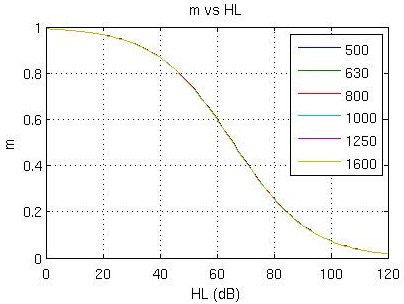
Figure 6. Maximum achievable information extracted as a function of hearing threshold. The same curve applies at all frequencies, not just the frequencies shown in the legend.
What we found quite reassuring was when we applied this same analysis to sentence material based on the Bamford-Kowal-Bench (BKB) and City University of New York (CUNY) tests, and then to consonants in the form of the vowel-consonant-vowels (VCVs), we got very much the same curves. We think this is, at least on average, a reasonable indication of how much information hearing-impaired people can extract from speech. It is why we fit cochlear implants to people with severe and profound hearing loss, because the ability to extract information, even when we make speech as audible as possible, is so low when presented acoustically.
We ended up with a series of curves showing the effective audibility (Figure 7), meaning that as the sensation level increases, the amount of sound that people can actually use increases. However, the more hearing loss you have, the less it increases.
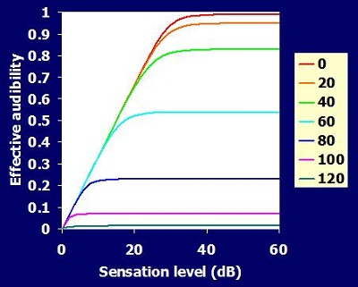
Figure 7. Effective audibility as sensation level increases. The colored lines indicate hearing level from 0dB (red) to 120dB (green). Audibility decreases as hearing loss increases.
Psychoacoustics
It is a bit disappointing in a way that, after all these years, we are still prescribing hearing aids on the basis of pure-tone thresholds. What aboutthe many psychoacoustic parameters that we know are affected by hearing loss?
We have also measured outer hair cell function through click-evoked otoacoustic emissions. We estimated frequency resolution from psychoacoustic tuning curves and from a test of dead regions known as the TEN test that I will say more about soon. We have also measured cognitive ability, and of course, age.
Psychoacoustic tuning curves give you an idea of how sharply tuned the cochlea is to signals at a range of frequencies. If the signal is 1,000 Hz, we can see in Figure 8 that it is best masked by a narrow band masker also tuned to 1,000 Hz. That is what we expect for a normal functioning cochlea. As the masker moves away from the frequency, either up or down, then the masker becomes less effective.
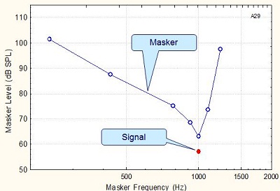
Figure 8. Tuning curve for a signal of 1,000 Hz in a normal cochlea.
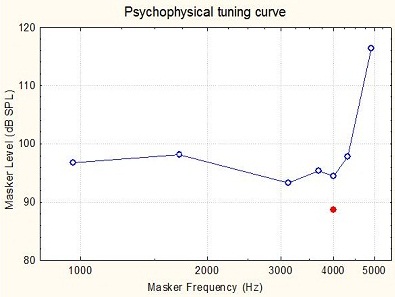
Figure 9. Tuning curve for a 4,000 Hz signal in a damaged cochlea.
For somebody who has a non-functioning cochlea at 4,000 Hz, the curve might look wide and flattened (Figure 9). The signal is at 4,000 Hz, but the most effective masking frequency is at 3,000 Hz. In other words, it seems that the person is detecting this 4,000 Hz signal, yet not at the 4,000 Hz place in the cochlea, but at the 3,000 Hz place in the cochlea. That is why a 3,000 Hz masker is actually slightly more effective than a 4,000 Hz masker. So the psychoacoustic tuning curves tell us about the sharpness of the tuning, and they also tell us about the likelihood of the person listening at places in the cochlea other than where the signal is, presumably because the inner hair cells are not sufficiently functioning in order to send a good detection signal to the brain at the original frequency in the cochlea.
There is, of course, a very specific test of dead regions from Moore and colleagues (2004) called the TEN Test. There is some evidence from the same research group in Cambridge that one needs to take this knowledge of dead regions into account in determining whether it is worth amplifying at each frequency. There is also some conflicting evidence suggesting that hearing thresholds are sufficient, and we wanted to investigate that.
The basilar membrane has an excitation pattern as a function of position along the cochlea. What happens if we have a dead region of the cochlea (i.e. no functioning inner hair cells)? Let’s suppose we put a signal in at a frequency that produces a specific excitation pattern with a peak at one place in the cochlea. Normally, that would get picked up most sensitively by nerves connected to this area in the cochlea and the adjacent frequencies. But if this high-frequency region of the cochlea is all dead, then the person is actually listening to parts of the cochlea that are tuned to lower frequencies.
If we were to put a masking sound in for the person with normal hearing, the masking sound would have no effect if the excitation from the masker is lower than the peak excitation from the signal. For the person who is actually listening in a frequency range outside the target frequency due to dead regions, the excitation from the signal where it is being detected is lower, so the masking sound may now mask the tone, so the input level would have to be increased when the broadband masking sound is applied. That is the basic concept: Apply a broadband masking sound and then look at what the threshold of the tone is. If it is higher than you would normally expect, it suggests that the person was listening elsewhere in the cochlea. The test is called the ‘Threshold Equalizing Noise Test’ or TEN Test, which is a very clever acronym, because the criterion is that the threshold rises 10 dB above the masking level of the noise.
We have looked at a comparison between the TEN Test and the tuning curve test, and in many cases, both tests agreed that the region of the cochlea was alive. In several cases, they agreed that that region of the cochlea was dead, that is no functioning inner hair cells. But there were some regions of disagreement, where one test said the region was alive and the other said it was dead. Sometimes you will find that you cannot complete one or other of the tests. This is because the masking sound gets too loud for the patient to stand it before it gets intense enough to mask the signal. So both tests will produce some uncertain results from time to time. Maybe we did not do the psychoacoustic tuning curves with the best possible stimuli. We are still scratching our heads as to why we did not get a good agreement there.
One of the problems in this work is that everything is correlated with everything else. We found significant correlations between the hearing thresholds, the sharpness of the tuning curves, the outer hair cell functioning as evidence by otoacoustic emissions strength, the results of the TEN Test, people’s cognitive ability and their age. This applied both at 2 kHz and 4 kHz. Correlations were also present at lower frequencies, but were less strong.
When all these factors are correlated, how do we know what factor is causing what? More specifically, can we make a better prediction of intelligibility if we make use of the psychoacoustic results?
The answer is, yes, we can predict intelligibility just a little bit better if we know about frequency selectivity. In our judgment, the advantage was not sufficiently great to cause audiologists around the world to be spending time measuring frequency selectivity; we did not think that it contributed very much to the ability to prescribe a hearing aid. If the aim of the hearing aid is to maximize intelligibility, and the psychoacoustics do not let us significantly increase our ability to predict speech intelligibility, then we think it does not add much to the hearing aid fitting process.
Why are thresholds so important and related to everything else? We think the mechanism is like this: as people get older, they develop hearing loss, and also their cognitive abilities decline (on average). Reduced functioning of the outer hair cells reduces the sharpness of the tuning curve, reduces the level of the otoacoustic emissions, and also cause elevation of the TEN Test results. Degradation of the inner hair cells causes further, sometimes marked, elevation of the TEN masked thresholds.
Hearing loss may or may not also produce a cognitive decline, as people are increasingly shut off from those around them. That is a very interesting question that we cannot answer yet. Of course, age by itself does not cause anything. Age causes cardiovascular problems and other physiologic problems. They, in turn, cause variations inside the cochlea, such as the degradation of outer hair cells and the stria vascularis, mechanical changes, a stiffer cochlea and perhaps reduced cognition as well. These things then cause the observed changes in tuning curve sharpness, otoacoustic emissions, TEN strength, and the straightforward audiogram. We think that is the mechanism underlying it. The end result is that, when you know about the hearing loss, you can then make predictions about these other parameters to a sufficient degree to do a reasonable job of fitting a hearing aid.
Intervening factors are many: frequency selectivity, temporal resolution, central auditory processing abilities, and other things that we probably have not even thought of yet. But at least if we know the hearing thresholds, we can make some predictions about speech perception. Of course, age is associated with degradation of all these other quantities.
I am now going to hand it over to Dr. Gitte Keidser to talk about some empirical findings.
Factors Affecting Prescription
Dr. Gitte Keidser: Hello, everyone. I am going to talk about the factors that will affect the NAL-NL2 prescription.
After the release of NAL-NL1, we received comments from clinicians around the world suggesting that many clients would not accept the overall gain prescribed by NAL-NL1. To study this further, we looked at the gain preferences by 187 adults who had taken part in various research projects that we had conducted here in Australia (Keidser, Dillon, Carter & O’Brien, in review). For each of these individuals, we had a real-ear insertion gain measurement of their preferred or fine-tuned fitting for listening to normal conversational input levels.
Figure 10 shows the average selected overall gain relative to that prescribed by NAL-NL1. The gain variations are shown separately for females and males, for new hearing aid users and experienced hearing aid users with a mild, moderate, or severe hearing loss. Negative values indicate that the subjects preferred less gain than prescribed. Across the board, our subjects preferred 3 dB less gain than prescribed by NAL-NL1, which means that NAL-NL2 prescribes 3 dB less overall gain than NAL-NL1.
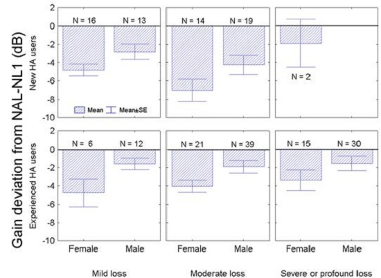
Figure 10. Preferred gain deviation from NAL-NL1 by new and experienced hearing aid users with mild, moderate and severe to profound hearing losses.
You may have noticed that whether the hearing aid users were new or experienced, and independent of what the degree of hearing loss was, the females tend to prefer less gain than the male hearing aid users. The difference was, on average, 2 dB, and that difference is statistically significant. Based on this finding, NAL-NL2 prescribes 2 dB higher gain for males than for females if you enter the gender of your client into the fitting software.
Finally, we found that there was no difference in the gain preferences between new and experienced hearing aid users with a mild hearing loss. However, new hearing aid users with a moderate hearing loss did prefer significantly less gain than did experienced hearing aid users with a moderate hearing loss. Therefore, we have introduced an effect of experience in NAL-NL2.
Experience was specifically investigated in one study that we did (Keidser, O’Brien, Carter, McLelland & Yeend, 2008). We looked at the gain variation from the prescription by new hearing aid users, and by experienced hearing aid users. We found that increasingly less gain was preferred by new users as the degree of hearing loss increased. For the experienced hearing aid users, the gain variation was relatively constant around minus 3 dB. So on this basis, NAL-NL2 does prescribe different gain adjustments for new hearing aid users, depending on the degree of hearing loss.
In Figure 11, the green broken line shows the net difference in gain that is prescribed to new and experienced hearing aid users as the degree of hearing loss increases. No difference in gain is prescribed while the loss is very mild. We see an increased difference in prescribed gain across the moderate hearing loss range, and then we settle on a constant gain difference as the hearing loss becomes severe to profound. The reason for this is that we have no data to suggest that we should vary the gain even more for those with profound hearing loss. It also seems counterproductive to reduce gain further for those who need it the most.
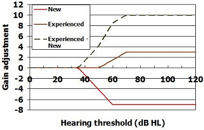
Figure 11. Adjustments to prescription to allow for experience level.
So what does that mean? That must mean that new users adapt to gain over time. What is that time period? We were able to follow 11 subjects with moderate hearing loss longitudinally (Keidser et al., submitted). We saw them for a period of three years, roughly every six months. At each appointment, we let them select their preferred program and the volume setting that they commonly used, and then we measured the overall gain. On average, these subjects increased their gain setting steadily over the first two years of hearing aid usage. After two years, their preferred gain setting was within the 95% confidence intervals of the gain preferred by experienced hearing aid users with a similar degree of hearing loss.
So far, we have talked about gain preferences for a medium input level, but what happens at low and at high input levels? Two studies conducted independently of each other both used a research device that logged information about the input level of the subjects’ environment, as well as the volume control settings that they selected in these environments (Smeds, Keidser, Zakis, Dillon, Leijon, et al., 2006; Zakis, Dillon, McDermott, 2007). Both studies showed that the subjects selected further gain reduction for an 80 dB input level, relative to the gain variation from the prescription they selected at a 65-dB input, but less gain reduction for a 50-dB input level. What that means is that they actually preferred higher compression ratios than those prescribed by NAL-NL1.
We have established that adults prefer 3 dB less gain for a 65-dB input level, and that they prefer a higher compression ratio than prescribed by NAL-NL1, which is achieved by reducing gain further for high input levels, but not for low input levels.
Other studies (Scollie et al., 2010) have suggested that children tend to prefer higher gain levels than adults for medium input levels. An increase in gain is more likely to lead to greater speech intelligibility at low input levels where speech may be limited by audibility. It is also less likely to cause a noise-induced hearing loss if introduced at low than at high input levels. Consequently, we are prescribing children with the same higher compression ratio that is prescribed to adults. For children, the higher compression ratio is achieved by increasing gain relative to the NAL-NL1 prescription, with more increase at low input levels, and not at all for high input levels.
An effect of age on prescribed overall gain has been introduced in NAL-NL2. The result did raise the question whether the difference in the preferred amount of gain between children and adults was due to age or whether it was because the hearing loss was congenital or acquired. We addressed this question by looking at data we had collected on 43 adults who were all fitted with the same type of hearing aids. Of these adults, 15 had a congenital hearing loss and 28 had an acquired hearing loss. There was no significant difference in the gain that they selected relative to the NAL-NL2 prescription across low or across high frequencies (Figure 12). So for now, we assume that age is determining whether children or adults prefer different amounts of gain.
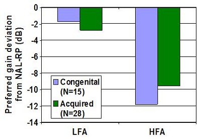
Figure 12. Preferred gain from subjects with congenital or acquired hearing loss for low and high frequencies. LFA= low-frequency average; HFA= high-frequency average.
Compression
I would like to go back to compression for a moment. The optimization process that Harvey talked about before does suggest that we should increase the compression ratio as the degree of hearing loss increases. We think that that will work fine, as long as we fit our clients with slow-acting compressors. However, many studies have demonstrated that high compression ratios combined with fast time constants can have a deleterious effect on speech understanding. In one study, we did find that people with severe and profound hearing loss, when fitted with fast-acting compressors, actually preferred closer to linear amplification, more so at low than at high frequencies (Keidser, Dillon, Dyrlund, Carter & Hartley, 2007). So in the derivation of NAL-NL2, we did develop two different formulas, one for slow-acting and one for fast-acting compressors. When we derived the formula for fast-acting compression, the gain from the optimization process was limited according to a mathematic function.
To sum it up, NAL-NL2 does prescribe different compression for slow and fast compressors for those with high degrees of hearing loss. There is no difference in the compression ratios prescribed for those with mild or moderate hearing loss with the two different compressor speeds.
Bilateral Loudness Correction
Bilateral loudness correction was introduced in NAL-NL1 to take bilateral loudness summation into account when we fit two hearing aids as opposed to one. Going back to the data on the 187 adults (see Figure 10), we had 136 subjects who were bilaterally fitted and 51 who were unilaterally fitted. We found that those who were unilaterally fitted selected significantly lower gain than did those who were bilaterally fitted. This indicates that the bilateral loudness correction in NAL-NL1 is too large. That is also supported by some newer data (Whilby, Florentine, Wagner & Marozeau, 2006; Epstein & Florentine, 2009).
In NAL-NL1, people who were unilaterally fitted were fitted with 3 dB more gain across the lower input levels, with an increase in gain up to about 8 dB for higher input levels. In NAL-NL2, this bilateral correction has been reduced to just 2 dB across the low input levels, increasing up to 6 dB for high input levels.
Effect of Language
The optimized gain at each frequency depends on the importance of that frequency to understanding speech. In tonal languages that are commonly found across the Asian and African countries, low frequencies are more important than they are in the English language. Therefore, two versions of NAL-NL2 have been derived: one for tonal and one for non-tonal languages. This was done by running the optimization process twice, one with an important function that was applicable to tonal languages, and one with an important function that was applicable to non-tonal languages.
The graph of Figure 13 shows an example of the difference in prescriptions for tonal languages, the blue line, and non-tonal languages, shown by the red line. Immediately, the difference does not seem to be great, but the effect of the difference is still to be verified in a clinical study.
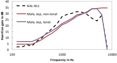
Figure 13. Comparison of gain for tonal (blue line) and non-tonal (red line) languages using male talkers.
In summary, NAL-NL2 differs from NAL-NL1 by prescribing a different gain frequency response and higher compression ratios, with the exception that we do prescribe lower compression ratios for those with severe and profound hearing loss if they are fitted with fast-acting compressors. Finally, the overall gain in NAL-NL2 depends on gender, age, experience with hearing aids, and language as well.
Examples of Prescriptions
In Figure 14, the colored full lines show the NAL-NL2 prescription for 50 dB, 65 dB, and 80 dB input levels; the broken line shows the NAL-NL1 prescription for a 65 dB input level. The prescribed curves are for a moderate, gently sloping hearing loss, shown on the left of the figure. As you can see, NAL-NL2 generally does prescribe a more smooth insertion gain curve. Relative to NAL-NL1, it prescribes sightly more gain at low and high frequencies, and less gain at mid frequencies.
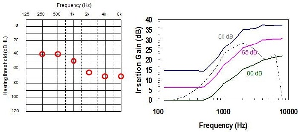
Figure 14. Example audiogram of a moderate sloping hearing loss (left) and the NAL-NL2 prescriptions at various inputs (color lines) compared with previous NAL-NL1 prescription (dashed line).
Similarly, for a flat hearing loss, NAL-NL2 has a more smooth prescription target and more gain is prescribed at low and at high frequencies than at mid frequencies, relative to NAL-NL1 (Figure 15). Looking at a steeply sloping audiogram (Figure 16), the main difference is at the high frequencies, but again, slightly less gain is prescribed at the mid frequencies. And for a ski-slope hearing loss (Figure 17), we have a smoother target across the high frequencies with more high-frequency gain prescribed than NAL-NL1, while less gain is prescribed at the mid frequencies. Finally, for a reverse sloping hearing loss (Figure 18), the main difference is in the low frequencies, where NAL-NL2 prescribes more gain than NAL-NL1 and in the high frequencies where NAL-NL2 prescribes less gain than NAL-NL1. Again, we have a more smooth insertion gain target.
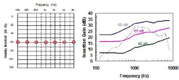
Figure 15. Comparison of NAL-NL2 to NAL-NL1 prescriptions for a flat moderate hearing loss.
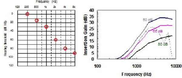
Figure 16. Comparison of NAL-NL2 to NAL-NL1 prescriptions for a steeply-sloping hearing loss.
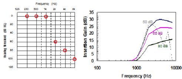
Figure 17. Comparison of NAL-NL2 to NAL-NL1 prescriptions for a ski-slope hearing loss.
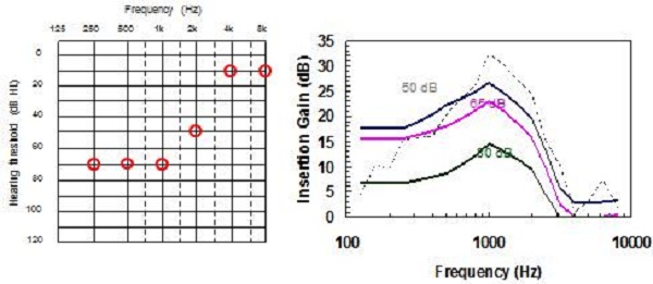
Figure 18. Comparison of NAL-NL2 to NAL-NL1 prescriptions for a reverse-slope hearing loss.
Dr. Harvey Dillon: Earl Johnson and I published a paper last year (Johnson & Dillon, 2011) showing a comparison of NAL-NL2 relative to NAL-NL1, DSL m[i/o], and CAMEQ2-HF. We applied a loudness model and also the speech intelligibility model to each of those prescriptions and to seven different audiograms.
For a flat, moderate hearing loss, the different prescriptions look pretty similar in terms of how much loudness they would prescribe. We start to see some differences, however, when we get to more steeply sloping losses. Where hearing loss is most severe in the high frequencies, NAL-NL2 gave up more easily on providing gain than any of the other prescriptions. CAMEQ-HF always tries to provide audibility at all frequencies. If it could talk, NAL-NL2 would have said that high frequency gain produces diminishing returns for intelligibility while increasing loudness, so it gave more emphasis to the mid and low frequencies instead.
That is the essential difference. In the reverse slope loss where the most severe loss is in the low frequencies, NAL-NL2 tends to more give up than the other prescriptions. That is as a consequence of that hearing loss desensitization being built into the derivation. In terms of loudness, CAMEQ2-HF was pretty similar in loudness to NAL-NL1, and DSL and NAL-NL2 gave lower overall loudness. We do not see very large differences between the four procedures for the SII, or prediction of intelligibility.
Pediatrics
We have not said much about children, but we have a longitudinal study under way at the moment led by Dr. Teresa Ching. We have collected data on about 500 children, looking at everything that happens to them as far as amplification is concerned, as well as their outcomes for language. The data is now complete up to age three, and almost complete at the age-five data measurement point.
Included in this experiment was a randomized allocation of half the children to get the NAL prescription, which, when we started, was NAL-NL1. We since have changed over to NAL-NL2, and then the other half of the subjects got the DSL prescription, which again, when we started was 4.1, and now is DSL m[i/o]. So far, we have found no difference in the language outcomes between the NAL-NL2 and the DSL m[i/o] groups. There are still some differences in the prescriptions, but as our groups have gone through successive iterations, the formulas have come somewhat closer together. It appears that there are no consequences of the differences in prescription for language outcomes of children, at least up to the age of five years.
I would like to mention just two things to finish. The first one is that insertion gain is the heart of the NAL-NL2 prescription. The audiogram gives rise to the insertion gain. The insertion gain, as Gitte said, is also affected by experience, the type of language, gender, age of the person, speed of the compression, and whether the hearing loss is bilateral or unilateral. All of those parameters let us calculate the insertion gain. From the insertion gain, we can then calculate the real-ear aided gain, the coupler gain, the gain in an ear simulator, and it also influences the maximum output of the hearing aid
Trainable Hearing Aids
There is a development which we think will take a little bit of pressure off measuring whether gain-frequency responses have achieved the prescribed responses. If the hearing aid software can do a reasonable job of getting close to the prescription, then the trainable hearing aid offers the potential for the user to do the fine-tuning rather than the audiologist.
The hearing aid takes notice of the adjustments the wearer makes to the hearing aid, remembers them and uses them to fine-tune the hearing aid. The most sophisticated trainable hearing aids also measure and remember the acoustics of the situations in which those adjustments were made and use those measurements to help interpret the adjustments. Over time, the hearing aid can build up a picture of what the person likes in different environments, and it can then make predictions about new environments.
For example, suppose a person adjusted the volume control and the hearing aid measured the input level. After the person had been in six environments, we would have six observations of how much gain the person liked for each of those input levels. The hearing aid could then do some curve fitting (Figure 19). What does that curve tell us?
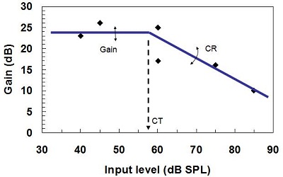
Figure 19. Training gain, compression ratio, and compression threshold for trainable hearing aids. The diamonds show input levels of six different environments.
Well, the first thing it tells us is the compression threshold, or the point at which the gain starts to decrease. In this case (Figure 19), that is 57 dB SPL. The second thing that it tells us is how much gain the person wants below compression threshold. The third thing is how much the gain reduces as the input level rises above compression threshold. That, of course, tells us what the compression ratio is.
Just on the basis of the person adjusting the volume control, they have actually fine-tuned the hearing aid’s gain below compression threshold, the compression threshold itself, and compression ratio. We think this is a good development for hearing aids, which lets people fine-tune hearing aids in their own environment, by doing nothing other than adjusting their hearing aid in the usual way.
It is our challenge to develop the best prescriptive strategies and fit them the best way we know how. So choose carefully, and thanks for listening.
Question & Answer
When might we see NAL-NL2 targets incorporated in probe mic systems?
The NAL-NL2 prescription has been licensed to most of the manufacturers of probe mic systems. So very soon, if it is not in them already, is my answer.
How did maximum power output (MPO) change with the new prescription?
We have not changed our prescription much for MPO or saturation sound pressure level (SSPL) from what it was with NAL-NL1. We prescribe maximum output of the hearing aid from hearing thresholds. We did change some of the details of it, however. We think we allowed too aggressively for multichannel hearing aids, so there is now a smaller difference between the prescription for multichannel hearing aids and the prescription for when limiting is done on the whole signal rather than separately within each channel. That was a small change. We are still prescribing MPO based on threshold, not on measurement of discomfort level.
We did some careful research 12 or so years ago to try and answer the question, “Should we be measuring loudness discomfort level when prescribing maximum output?” We came to a convincing answer that, no, it did not add enough to the prescription in order to justify the time taken clinically.
Should we be using RECDs for adults just like we use for infants?
There is no absolute right or wrong answer to this. You can prescribe a hearing aid on the basis of insertion gain and verify it with the insertion gain. Or, you can prescribe a hearing aid on the basis of real-ear aided gain, and then verify it with a real-ear aided gain measurement. Or, you can measure the individual’s RECD and infer what the real-ear aided gain should be. Both for adults and infants, you can do it either way. We think just the balance of practicalities drives you in different directions for the two.
In the case of infants, it is pretty hard to get the infant to sit still while you have a probe tube in the ear without a hearing aid to hold the probe tube still. There is also a philosophical question to consider. We know that infants will have a very high-frequency canal resonance at 6 kHz when they are born. That progressively moves down to 2.7 kHz by the time they are five or six years of age. Is that something that we need to preserve in a hearing aid fitting, or do babies just have a high-frequency resonance in their ear canal simply because they have small ear canals, which they have because they have small heads, which in turn they have because they need to be born?
Well, I think the latter is probably right; in which case, there is no real point in recreating that high-frequency canal resonance. If we use a real-ear aided gain approach rather than an insertion gain approach, we will actually give them the same pressure at the eardrum as we would for an adult. So the practicalities of difficulty in measuring insertion gain and the philosophical argument of, “Do we really want to recreate that super-high frequency canal resonance?” push us toward real-ear aided gain for the infant.
Then it becomes a logistics question, “Is it easier to measure with a probe tube after you have fitted the hearing aid or do it before and measure the real-ear-to-coupler difference?” We think measuring the real-ear-to-coupler difference is easier. When it is not possible, it is actually not too unreasonable, I think, to predict the real-ear-to-coupler difference based on the age of the child.
For adults, I think insertion gain is easier, and it is less prone to errors. With insertion gain, it is a different measure. You only need one microphone, the probe microphone. You are not comparing a probe to a coupler microphone. There is less potential for a calibration error in your equipment to cause a problem.
So there is the long answer, long probably because there is no real right answer. The short answer is that we recommend real-ear aided gain, achieved by a RECD measurement for infants and insertion gain for adults.
References
Ching, T. Y. C., Dillon, H., & Byrne, D. (1998). Speech recognition of hearing-impaired listeners: Predictions from audibility and the limited role of high-frequency amplification. Journal of the Acoustical Society of America, 103(2), 1128–1140.
Epstein, M., & Florentine, M. (2009). Binaural loudness summation for speech and tones presented via earphones and loudspeakers. Ear and Hearing, 30(2), 234-237.
Johnson, E., & Dillon, H. (2011). A comparison of gain for adults from generic hearing aid prescriptive methods: Impacts on predicted loudness, frequency bandwidth, and speech intelligibility. Journal of the American Academy of Audiology, 22, 441-459.
Keidser, G., Dillon, H., O’Brien, A., & Carter, L. (In review). NAL-NL2 empirical adjustments. Trends in Amplification.
Keidser, G., O’Brien, A., Carter, L., McLelland, M., & Yeend, I. (2008). Variation in preferred gain with experience for hearing aid users. International Journal of Audiology, 47(10), 621-635.
Keidser, G., Dillon, H., Dyrlund, O., Carter, L., & Hartley, D. (2007). Preferred low and high frequency compression ratios among hearing aid users with moderately severe to profound hearing loss. Journal of the American Academy of Audiology, 18(1), 17-33.
Moore, B.C.J. & Glasberg, B.R. (2004). A revised model of loudness perception applied to cochlear hearing loss. Hearing Research, 188, 70-88.
Moore, B.C.J., Glasberg, B.R., & Stone, M.A. (2004). New version of the TEN test with calibrations in dB HL. Ear and Hearing, 25, 478-487.
Scollie, S.D., Ching, T., Seewald, R., Dillon, H., Britton, L., Steinberg, J., & Corcoran, J. (2010). Evaluation of the NAL-NL1 and DSL v4.1 prescriptions for children: Preference in real world use. International Journal of Audiology, 49(S1), S49-S63.
Smeds, K., Keidser, G., Zakis, J., Dillon, H., Leijon, A., Grant, F., Convery, E., & Brew, C. (2006). Preferred overall loudness II: Listening through hearing aids in field and laboratory tests. International Journal of Audiology, 45(1), 12–25.
Whilby, S., Florentine, M., Wagner, E., & Marozeau, J. (2006). Monaural and binaural loudness of 5- and 200-ms tones in normal and impaired hearing. Journal of the Acoustical Society of America, 119, 3931–3939.
Zakis, J.A., Dillon, H., & McDermott, H.J. (2007). The design and evaluation of a hearing aid with trainable amplification parameters. Ear and Hearing, 28(6), 812-830.