The Movin' Groovin' Outer Ear

Learning Outcomes

After this course learners will be able to:

• Give a brief explanation of how the Lantos scanning system works.
• Describe how jaw motion affects ear canal shape.
• Explain how pressure applied during scanning or impression-taking can affect ear shape.
• Describe the regions of compliance in the outer ear and ear canal.

Introduction

Thank you for your participation in the Lantos Technologies course, "The Movin' Groovin' Outer Ear: Visualizing Compliance to Help Inform Comfortable Fit."  This course covers recent research at Lantos on the dynamics and compliance of the ear carried out using our ear scanning system. I'm pleased to be able to share some of these research findings with you today.

If you're not familiar with Lantos, we make the only FDA-cleared 3D digital ear scanner. In this course, after I explain the Lantos scanning system and how it works, we will discuss why we should pay attention to outer ear dynamics and compliance. Using 3D motion images in subjects’ ears, I'll demonstrate ear dynamics with jaw motion. Next, we'll see how comparing and contrasting ear scans and ear impressions informs us where the ear has the most flexibility and how you might apply that to the design or to the modification of comfortable earpieces. We'll conclude with some information about how the ear canal reacts to applied pressure. Much of the content of this course will focus on the ear canal.

The Lantos 3D Scanning System

All the work I'm going to tell you about today was carried out using the Lantos 3D Scanning System. Although you can purchase the system, I would like to preface this talk by making it clear that this is a research presentation. Some of the information I will be sharing was conducted either using a "tricked-out" scanner or in-house software that isn't commercially available. We did this to get a better understanding of our system, the ear, and the interaction between our system and the ear. In the course of doing these studies, we've made some exciting discoveries. To begin, I'm going to walk through how a scan is performed, and then we'll watch a short video of scanning in action.

How It Works

The system uses a membrane (Figure 1) that is central to the experiments we will discuss today. After loading the membrane and the solution into the scanner, you place the membrane and the camera down the ear canal. There's a clear window at the end of the membrane so you can see exactly where you're going when maneuvering the camera. On the screen, there is a yellow circle that allows you to align the annulus of the tympanic membrane (TM) to that circle, sort of like a distance gauge to indicate when you're about four to five millimeters away from the TM. 

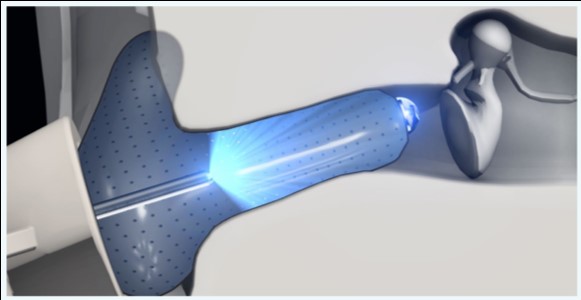
Figure 1. Membrane and camera in the ear canal.

Once you've reached the correct depth with the camera, the membrane gently inflates with a red water-based solution, and then the camera retracts. The camera emits a blue light that makes the inside of the membrane glow yellow. It glows yellow because the membrane is fluorescent, and the combination of that yellow light coming back to the camera and the red solution the light passes through lets the scanner measure the distance from the camera tip to the inside surface of the membrane that's right up next to the surface of the ear. As you scan, you move the camera first around the concha, and then down the ear canal. The software then converts the 2D images to 3D and stitches them together, by a process similar to taking a panoramic photo but in 3D (Figure 2).

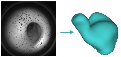
Figure 2. A collection of images like the one on the left are converted from 2D to 3D and stitched together into the complete scan.

The scanning process is shown in the following video; the person speaking is Erin Henry, our Director of Training.

Ear Dynamics and Compliance

Now that you have an idea of how the scanning process works, let's review the reasons why we should care about ear dynamics and ear compliance. First, I'd like to start with some definitions.

• Ear Dynamics: Ear dynamics refers to the motion of the ear, such as when the ear canal changes shape when a person opens or closes his or her jaw.
• Ear Compliance: Compliance refers to the flexibility or "give" that various parts of the ear have. For example, at the extremes, the earlobe is highly compliant, while the bony portion of the ear canal near the tympanic membrane has very low compliance. Compliance is the opposite of stiffness; something that is stiff is not compliant, and something that is compliant is not very stiff.

The terms ‘compliance’ and ‘dynamics’ are related in that a compliant substructure can move more easily in a dynamic situation. A dynamic ear canal can cause a hearing aid to move around or migrate, which can lead to feedback, inadequate amplification, as well as discomfort. In turn, the patient may become frustrated and experience diminished benefit, perhaps even outright rejection and return of the device.

One reason to understand the ear's compliance (or where it has "give") is to help design earpieces to be comfortable. For example, a typical hearing aid shell will be "waxed up" (digitally) around the aperture to provide retention and a good seal. However, this could potentially cause a sore spot or discomfort if it's done in the wrong spot or to an excessive degree. Knowing where the ear has "give" helps design devices, and direct modifications and remakes.

Ear Dynamics with Jaw Motion

When we open and close our jaw, our ear canal can change shape. Why is this? Let's take a detailed look at our anatomy.

To understand why the ear canal changes shape when we open and close our jaw, we need to look at the skull and the temporomandibular joint (Figure 3). The TMJ is unique in the body in that it's bilateral, but it moves as a unit. No other joint crosses the vertical plane of the body. The two joints on either side of the jaw are also unique because they both pivot and glide, and although there are a handful of others like this in the body (e.g., the wrist), there aren't very many. There is a disc that facilitates this motion as shown in Figure 4.

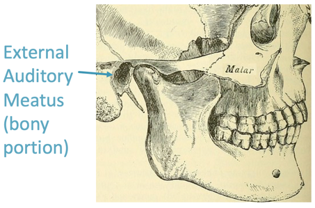
Figure 3. The skull, external auditory meatus (bony portion) and temporomandibular joint.

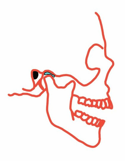
Figure 4. The mandible pivots and glides at the TMJ.

Take a moment and examine the TMJ on your own jaw. Find the back bottom corner of your mandible with your index finger, and next to it, place your middle and ring fingers right on the back of the mandible and open and close your jaw just a little bit, not quite an inch. You should be able to feel the pivot motion. Now, continue to open your jaw as far as it will go. You should notice the forward glide as the disc moves to the articular eminence.

What does this movement have to do with the ear canal? Take a look at the position of the bony portion of the ear canal relative to the TMJ (Figures 3 and 4). The ear canal lateral to the bony portion is made of soft tissue. As such, when the jaw moves forward during the glide portion, it pulls at the tissue of the canal because there's no air gap in between. There are various types of soft tissue. That is why the ear canal changes shape with jaw motion.

The shape change of the ear canal with jaw motion is well-documented. Oliveira and colleagues looked at impressions of 18 individuals in various states of jaw opening. In their study, they took impressions of the participants' ears with increasing numbers of tongue depressors between their teeth. They found that there is an increasingly larger change in the diameter of the ear canal from the front to the back as you open the jaw than there is from the top to the bottom. Looking at the graph in Figure 5, you can see that the inferior-superior change is relatively constant (yellow line), but the anterior-posterior width of the canal increases (blue line). Of course, it eventually levels off because we're not snakes and we can't unhinge our jaw to an incredibly wide proportion.

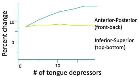
Figure 5. Percent change in diameter of ear canal with an increasing number of tongue depressors. (Adapted from Oliveira R. (1995). The dynamic ear canal. In: Ballachanda B, ed. The Human Ear Canal. San Diego, CA: Singular Publishing Group, pp. 83–112.)

The Lantos Experiment: Measuring Canal Motion in Response to Jaw Opening

Today, I'm going to show you images of two different subjects which we will refer to as Subject 1 and Subject 2.

Subject 1. Figure 6 shows some of the work that was done using in-house software that's not commercially available. In the dynamic view of the canal on the right, the ear canal widens when the jaw opens (Figure 6A). We are looking down the right ear canal. The anterior wall is where the most motion is, and it is moving towards the front of the face just like it would be if you were looking into the individual's ear from this vantage point. The red and blue image in Figure 6B is the full scan of the ear, and the light blue portion shows what part of the canal we're looking at in the dynamic view.

Figure 6A. Right ear canal during jaw opening and closing, Subject 1.

Figure 6B. Right ear full scan with region seen in Figure 6A animation shown in blue.

Figure 6C shows a heat map so we can quantitate this motion and how much the canal expands. At its widest opening, as indicated by the yellow-green color, the canal changes by about a full millimeter, or maybe even a little bit more. While a millimeter might not seem like a lot, it's actually around 10% of the diameter of a typical ear canal, so that's a pretty big motion in this particular case. 

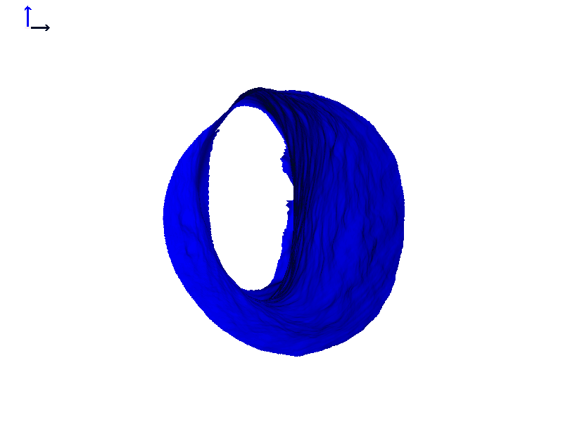
Figure 6C. Heat map of expanding ear canal; right ear, Subject 1.

In that same individual's left ear, the heat map does show a change, but it was not quite as dramatic as in the right ear (Figure 6D). These animations highlight the fact that ear canal shape change can be asymmetric and that the right and left ears can show different magnitudes of motion. If you're finding that a patient has a hearing aid or earmold that tends to not want to stay in place, it could be possible they have one canal that moves more dramatically when they speak or chew, as compared to their other one where the hearing aid stays put.

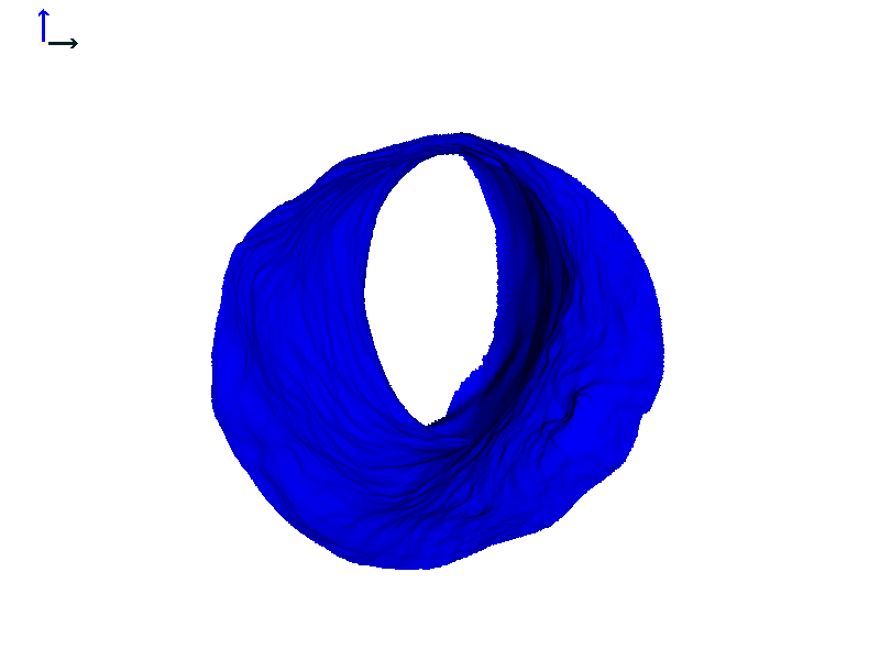
Figure 6D. Heat map of expanding ear canal; left ear, Subject 1.

Subject 2. Let's take a look at another individual that we will call Subject 2 (Figure 7). In this individual, there is also motion of both ear canals with jaw opening. In both cases, the expansion happens towards the front of the head or the face.

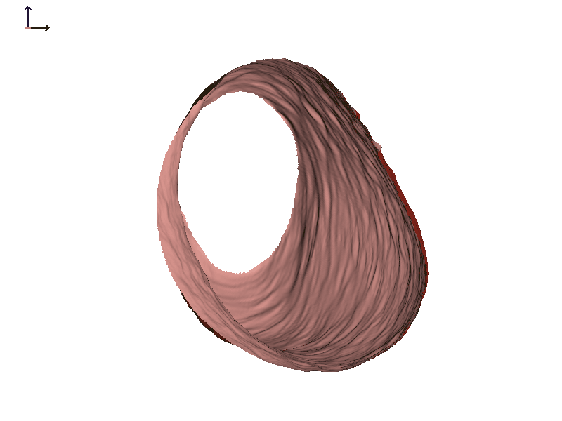
Figure 7A. Subject 2 right ear.

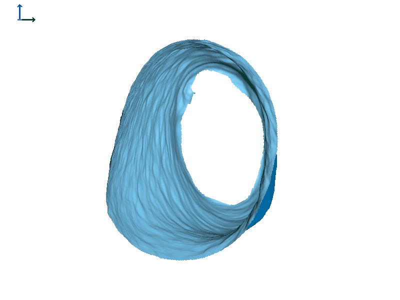
Figure 7B. Subject 2 left ear.

Figure 8 shows the ears of Subject 2 with heat map rendering. In this subject, the movement on each side is more comparable in magnitude than Subject 1, with perhaps a little more motion in the left ear (based on the colors in the heat maps).

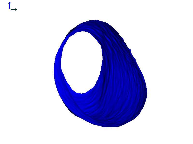
Figure 8A. Subject 2 right ear heat map rendering.

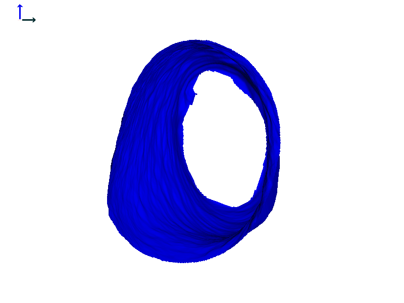
Figure 8B. Subject 2 left ear heat map rendering.

To recap before we move on, I showed you the anatomy of the TMJ and how the jaw's position can influence ear canal shape, which can affect different ear canals differently, even in the same individual. While you can get some information from the two states (the open and closed jaw), there is a lot more going on as one moves from fully closed to fully open, which begs the question "What is the appropriate reference state to begin with?" Finally, the difference in the canal diameter from fully closed to fully open can be around 1 millimeter. If you’re thinking of a pressure vent, 1 mm might not seem like all that much, but remember, this is an area larger than a 1 mm diameter circle and is 10-15% of the ear canal’s diameter.

Compliance: Comparing Scans and Impressions

Now that we've talked about dynamics, we will move on to compliance. The next study I'm going to share was done by comparing ear impressions and ear scans to each other. In this case, both the scans and impressions were taken in a relaxed close jaw state. We did not make the ear move by asking subjects to open and close their jaw. These are static scans and static impressions compared to each other. Before we discuss that experiment, though, let's travel through the history of ear imaging.

History of Ear Imaging

As with direct ear scanning (like the Lantos scanner which had its origins in intraoral or dental scanning), impression taking also began with the teeth (Figure 9). Dental impressions were made from wax and plaster back in the first half of the 19th century. The first reported ear impression was made in 1890 for an ear trumpet, as in this era there wasn't any kind of electronic hearing aid with amplification. Wax was used to make that first known impression. Plaster of Paris, which seems to make more sense for dental impressions, was also occasionally used for ear impressions. I would imagine that in a particularly tortuous canal, that would be tricky, especially when it came to removing a plaster impression. In 1946, the powder/liquid acrylic ethyl methacrylate impression material was introduced, which was used for quite a long time. In fact, to this day, there are still fans of the powder and liquid, and hearing aid and earmold labs still receive such impressions.

Figure 9. Ear imaging timeline.

The first ITE was introduced in the early 1950s, and also around this time, silicone as an impression material was introduced but not widely accepted for about 20 years. The ITEs and earmolds that were made during this time period were all direct pours. A physical negative of the impression was made and the hearing aid shell for the earmold was poured from that. It was similar to a casting process, and this technique is still used today for some applications. Desktop impression scanning came about in the late 1990s to early 2000s, and digital shell modeling and 3D printing revolutionized how custom hearing aids were produced.

In 2018 at the AAA conference in Nashville, both Lantos and Otometrics demo-ed robust direct ear scanning. Both companies had presented products at conferences before, but in 2018, the scanners shown at the conference went beyond just prototypes. Today, both scanners are available for purchase for your audiology practice. 

If you'd like more information about the history of ear impressions, I recommend taking a look at the series of Wayne's World articles at HearingHealthMatters. Wayne Staab has done a terrific job covering the history of impressions. He also has a lot of good articles on ear canal anatomy, hearing aids, and other related topics.

Aperture of the Ear Canal

The aperture to the first bend region is where the seal of a hearing aid or an earmold is made. It's an important region to model properly when the lab is designing a hearing aid. The next experiment I want to tell you about focuses on that aperture to first bend region, and it deals with comparing static 3D images, namely scans and impressions. We took 68 matched pairs of scans and impressions, we overlaid them, and we minimized the average distance of the aperture in the canal. Then we measured the difference between them in four directions at the aperture: superior, anterior, inferior and posterior. On the next few slides, superior will be represented in blue, anterior in red, inferior in green, and posterior in yellow. In those four directions, we compared how far apart the scan dimensions were to the impression dimensions.

The Lantos Ear Scanning Process

As a reminder, while you might expect there to be no difference between scans and impressions, that's not necessarily going to be the case. The two methods capture the ear in different states.

The Lantos scanning process is a contact method in that a fluid-filled membrane is used, and it's the inside surface of the membrane that contacts the ear that is scanned. The membrane is gentle but it does remain filled for the whole scan. The filled membrane serves as a proxy for someone having a hearing aid, an earmold, or another device in the ear, and the shape the ear adapts to is where it has the most compliance.

Ear impressions are also a contact method for getting the ear's geometry. There's a bit more pressure when the silicone is being injected into the canal, but since the impression material doesn't set right away, the ear still has a chance to relax a little bit after that material is injected. Neither method captures the ear without influencing it though. They're both contact methods, but they affect the ear shape in slightly different ways.

Aperture Compliance with Inflation

Figure 10 shows one example of a comparison of a right ear scan (in pink) to a right ear impression of the same individual's ear (in blue). They're geometrically lined up as if we are looking down that right ear of this individual. In this case, the scan (pink) is wider than the impression (blue) in the posterior direction. In the superior-inferior direction, the scan is narrower (shorter) than the impression.

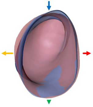
Figure 10. Comparison of right ear scan in pink and impression in blue.

Looking at all 68 matchups, we can see trends (Figure 11). I've made histograms for each direction where the colors of the bars match the locations around the ear, as shown in the previous image. Along the x-axis of each histogram is the displacement relative to the impression. The black bar indicates where zero is no difference. If the peak of the histogram falls on the left side, that means that the scan is a little bit smaller than the impression. If the peak of the histogram is on the right side, the scan is larger in that aspect.

In the superior aspect (blue), there's a little bit of a contraction on average (although not in every case). In other words, the aperture is not as tall in the scan as it is in the impression. In the anterior direction (red), the histogram is on the right side and falls greater than zero, so the scan is wider than the impression towards the front. In the inferior aspect (green), there is not much difference between scan and impression measurement, and the histogram is pretty well distributed about zero. Towards the posterior (yellow), there's also a bit of an expansion, so the scans are wider than the impressions, but it is not as extreme as towards the front (anterior).

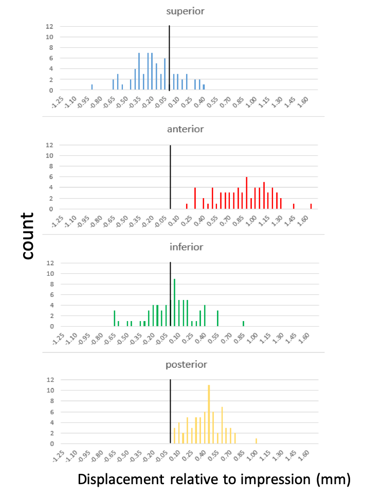
Figure 11. Histograms of all 68 matchups.

By overlaying 68 pairs of scans and impressions, we've discovered that with membrane inflation, the aperture tends to expand the most to the front of the canal and slightly to the back with little or no change at the top or the bottom. Figure 12 shows an exaggerated ear canal with the shape of a idealized, typical scan shown in red and the shape of a idealized, typical impression relative to that scan shown in blue. Interestingly, what we see here in the aperture using comparison of static scans and statistics is similar to what happens with the jaw motion. When we were looking at the jaw opening, that was a little bit deeper into the canal (between the first and the second bend region). There, the greatest change with jaw opening was towards the posterior also. In this case, we're looking a more distally in the canal at the aperture. The ear canal at the aperture in response to having something in it (i.e., an inflated membrane) opens up on average mostly in the front to back direction and does not open much (and even contracts a bit) in the top to bottom direction.

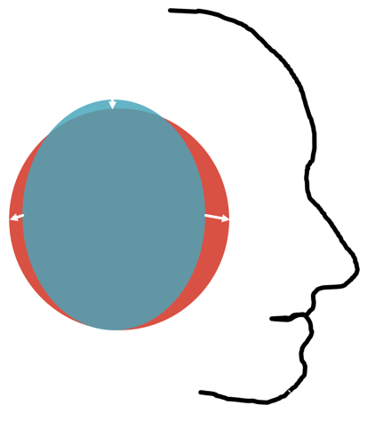
Figure 12. Exaggerated average ear canal aperture in scans (red) and impressions (blue).

What does this mean for hearing aid design and for hearing aid modification? The aperture appears to be less compliant in the inferior-superior aspect than in the anterior-posterior aspect. If a patient is complaining of a nonspecific pressure type discomfort and is not able to pinpoint a location, try grinding down the superior-inferior parts of the hearing aid or that earmold. If the lab has applied a digital wax-up, they probably did that evenly around the circumference of the device at the aperture. If it's causing discomfort, it may be necessary to take it down a bit. Taking it down at the top is less likely to sacrifice the seal than removing material at the front or the back.

Ear Reaction to Applied Pressure

Next, I'm going to demonstrate what happens when you apply pressure to the ear. But first, we will review some anatomy. When you were studying to become an audiologist, you may have studied pictures like the ones in Figure 13. You may have learned that the ear canal is half cartilaginous and half bony. Notice that the two pictures in Figure 14 show a very different ear canal anatomy. Imagine pushing on the pinna on the ear drawn on the left with your open palm versus pushing on the pinna drawn on the right. What could happen to the ear canal when you do that? In the left image, you see a lot more bone directly contacting the ear canal, but in the right image, you see more soft tissue almost all the way to the eardrum, and more of a gradual transition from soft tissue to bone.

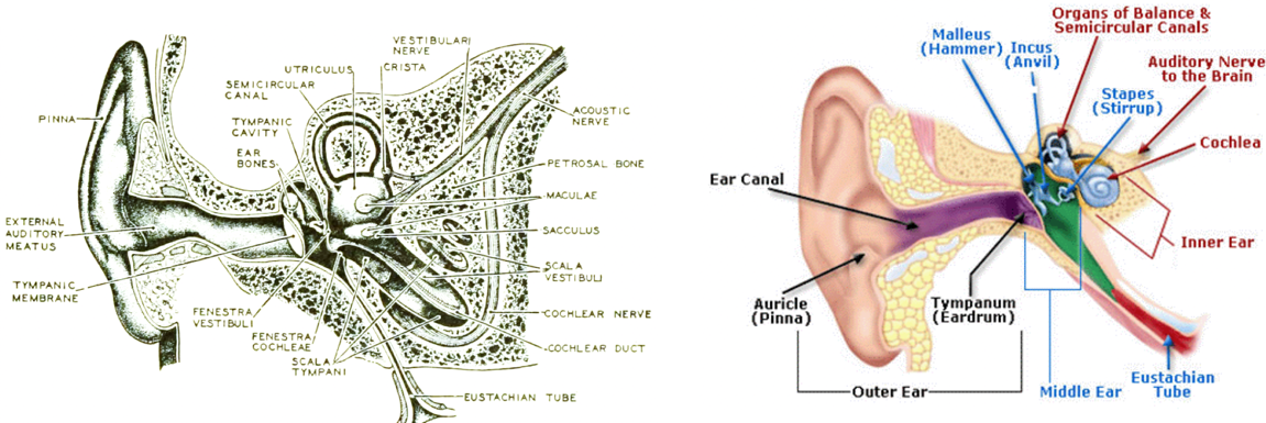
Figure 13. Two alternate ear canal anatomy renderings.

I hope what I have to show you next, from both publicly available imaging studies as well as from Lantos experiments, will give you a clear picture of the behavior of the tissue that's surrounding the ear canal.

CT Scan Example 1

First, let's take a look at some CT scan images that I obtained from a public database called radiopaedia.org (Figure 14). You may already know this, but in a CT scan, the bone shows up as white. This particular series was annotated by the radiologist who contributed it to the database. We're looking at an axial image, which by convention is shown from the direction of the patient's feet. The patient is lying supine on his or her back, their face is at the top of the image, and we're looking at that individual's left ear because they're lying with their feet towards us. 

Figure 14. CT scan example 1.

What you'll see is a series of stacked images that go from the bottom up, and they are going to loop. What I want you to look at is how the ear canal crawls from the pinna to the middle ear. It will move from right to left as the images stack up. Another thing to keep in mind is that in general, ear canals point up a bit. If these ears are in a patient's head, the ear canals are pointing in an upward direction, so that's why you're going to see that crawling motion of the ear canal as we go from the bottom to the top. You will see the canal and the first bend followed by the second bend. You can see how close the mandible is to the second bend region. It shouldn't surprise you that the tissue around the first bend is soft tissue, it's all surrounded by gray since you're accustomed to straightening the canal when you look into the ear with an otoscope. I want you to pay close attention to where that second bend is made. The bend occurs before the canal becomes completely bony.

CT Scan Example 2

Our second CT scan example shows both ears (Figure 15). While the previous example was that of a normal individual with no pathologies, this CT scan is from a six-year-old who had meningitis and subsequently had ossification of the semicircular canals, but not the cochlea. In children, ear canals are more level and don't point up as much. In a six-year-old, they're starting to approach a more adult-like shape.

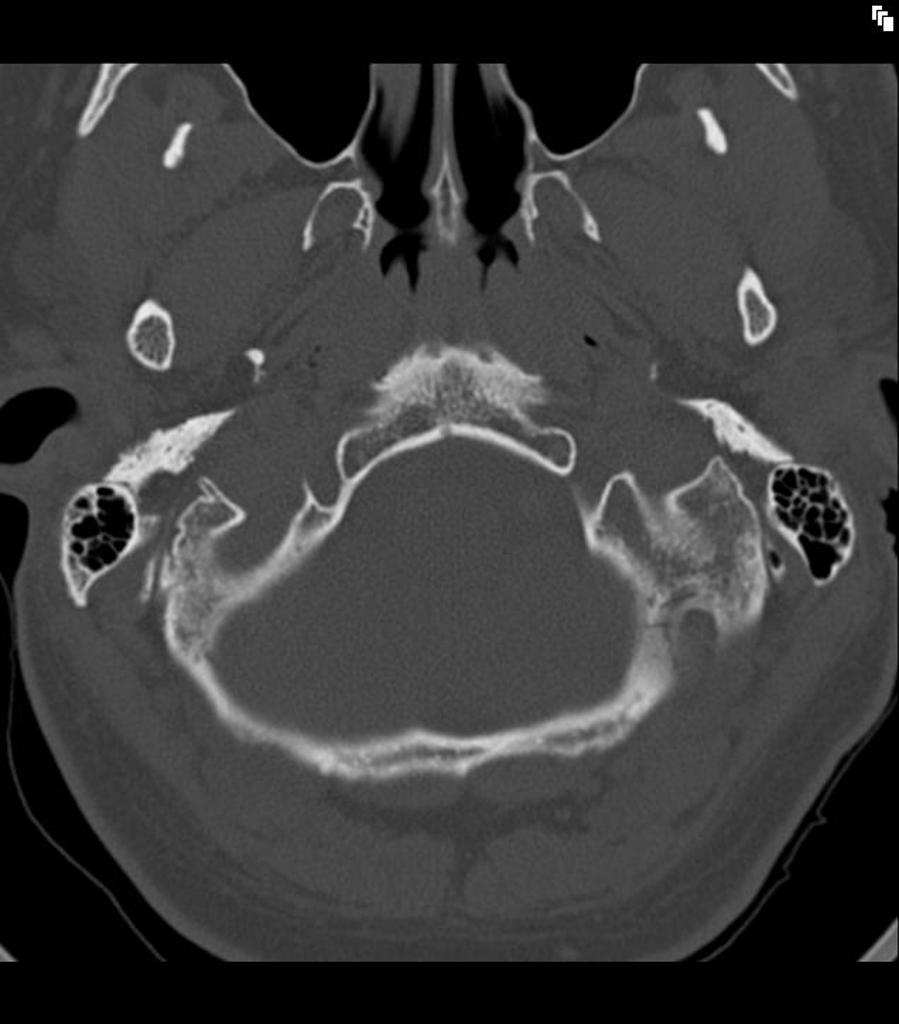
Figure 15. CT scan example 2, 6-year-old.

If we look in the left ear again, we can watch that canal crawl up as we're looking through the series of stacked images. You can see the first bend, and the second bend in this set is within soft tissue, at the bony-cartilaginous junction. You can see that the mandible is so close to the ear canal.  

Effect of Pressure on Ear Canal Shape

Now that we have seen the evidence from imaging studies, next I'm going to talk about what we see with the scanner. At the beginning of the talk, I mentioned that in order to record some of the 3D ear animations, we use either internal software (as I showed with the jaw motion movies) or a "tricked-out" scanner (Figure 16). The next experiments I am going to talk about were done with the latter. A few years ago, we outfitted a scanner with a pressure transducer (pressure measuring apparatus). We also used a special version of the scanning software that allowed us to scan multiple times without deflating and re-inflating the membrane.

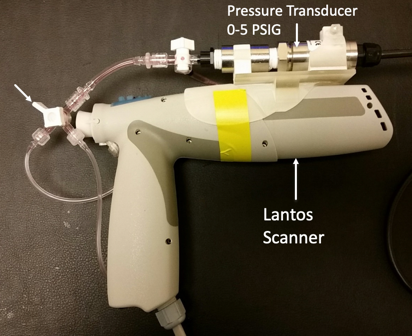
Figure 16. Scanner with pressure transducer coupled to absorbing medium fluid reservoir.

The experiment went as follows: the audiologist/operator scanned a subject's ear, targeting a different pressure with each scan. The way she would adjust the pressure was by varying the amount of force applied with the hand holding the scanner against the ear, but not so much that it was uncomfortable for the subject. The feedback was auditory. We found it was difficult to have the operator both watching, trying to scan, and at the same time, look in a different place and monitor an on-screen pressure reading. As such, we recruited a third person to read and call out pressure values in real-time. This way, the operator knew whether to push a bit or to release. (We didn't want the subject moving his or her jaw and talking because that would change the canal shape, as we learned.)

The x-axis in Figure 17 is time. What you're seeing is five different scans conducted at five different pressures. The pressure being measured is that of the fluid inside the membrane. Note these pressures are quite small (1 PSI or less). It's actually difficult to maintain a pressure of 1 PSI or above, which is more pressure than you would ever use in a real scanning situation. For reference, your car tire pressure is around 35 PSI, so 1 PSI would be a flat tire. The pressures that you use when performing tympanometry/immittance measurements are on the lower part of this scale. To be clear, we're measuring the pressure that is being achieved by the operator. For the duration of the scan, that operator is trying to maintain a 0.6 PSI. All the while, another person is calling out to let them know "too much", "too little", or is calling out the pressure measurement so the operator can adjust accordingly. You can see that the pressure is not absolutely constant throughout the scan, as maneuvering around bends and maintaining an exact pressure is difficult.  It is more difficult when targeting a higher pressure.

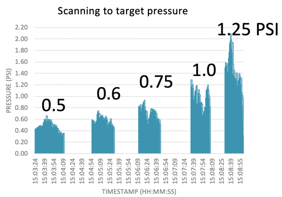
Figure 17. Scanning to target pressure.

Straight vs. Full Ear Membrane

It's important to note that these experiments were done with our old membrane design, which was a straight design (Figure 18). The straight design can only scan the canal in the proximal concha, which is good enough to create an ITC-sized device, but not anything bigger than that. An ITC, a CIC, or a canal earplug could all be made from a scan using this straight membrane. When you look at the images that I'm going to show you, you're not going to see the cymba concha because, with that membrane, we weren't capturing it. This membrane was also made of a different material, and the studies that we did helped us to design this what we call a full ear membrane by optimizing its shape and its performance in material.

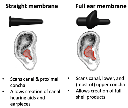
Figure 18. Straight vs. full ear membranes.

Coming back to the experiment, Figure 19 shows the corresponding scans that were obtained at each of the pressures shown in Figure 17.

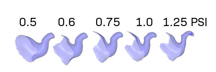
Figure 19. Scans obtained at different PSI.

In Figure 20, the scans in Figure 19 are put together into an animation. To orient you, the tragus is at the bottom, and the antitragus is facing us. If I showed it to you as it is oriented in an upright head, you wouldn't be able to see the first and second bend so we're viewing it as if the person is lying on their belly with their nose to the ground. This video loops. Notice that it goes from low pressure to high pressure. Also, notice how both the first and the second bends become a little bit more acute. It is similar to an accordion motion the way that the ear canal is getting compressed.

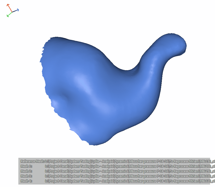
Figure 20. Subject MB, left ear.

As more pressure is applied, both the first and second bends become sharper. For the ears we looked at in our experiments, the ideal pressure is somewhere around 0.6 to 0.7 PSI. This tells us that you can affect the canal quite dramatically by pushing on the ear. We know this from experience when testing hearing that canal collapse can occur when testing with supra aural headphones if your patient has a narrow canal. Viewing these images, perhaps you can better envision what that canal collapse might look like. It would be interesting to repeat this experiment with the jaw open and then see how that first and second bend region responds to external pressure.

Here is another individual's ear (Figure 21). This is a wider, slightly straighter canal. You can also imagine while you're looking at this where the bony region might be by observing where it does not change shape very much.

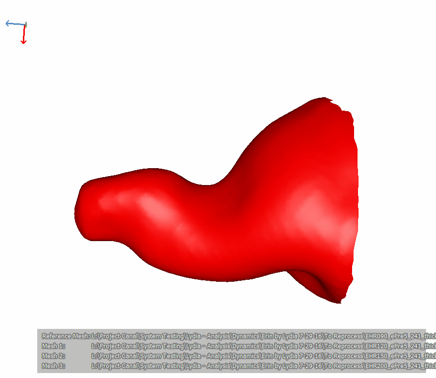
Figure 21. Subject EH, right ear.

These experiments were useful to us when it came to designing the current concha capturing membrane. They helped us to redesign the membrane through both changes in the material and the shape, and by adding what we call a nose to the membrane which is what's used to capture the cymba concha. We also added material that is better at absorbing applied pressure without deforming the ear. In fact, it is a lot more difficult to do this experiment with the new membrane because it's harder to achieve those excess pressures. Finally, the information we gleaned from these experiments also helped us develop our training program.

Summary and Conclusion

Let's revisit the two illustrations of the ear canal that we saw earlier in Figure 13. As a result of this presentation, I hope you'll agree that the image on the right of Figure 13 can better account for the dynamics and the compliance of the ear when it comes to both CT scans of the type of tissue surrounding the canal, as well as the experiments we conducted applying pressure while scanning. I would say that the image on the left has too much bony region. In retrospect, it's not completely surprising because when you do otoscopy, you do pull on the ear to straighten the canal. It’s also worth keeping in mind that when you take an impression, most of the canal you see in the impression (even in a pretty long impression) is soft tissue. Sometimes you can see the bony-cartilaginous junction of the impression, which is recognizable by the texture where the ceruminous pores end, but not all impression materials and not all ears will show that detail.

What does this mean to you? I know that some audiologists like to flatten impression material in the ear when it cures. If that happens to be you, just keep in mind that you could be changing the canal shape to an unnatural one, at least momentarily, without realizing it. Even though the material is soft and the ear can relax, you might inadvertently be creating gaps with the compression because if you push hard enough, you'll get that accordion effect. You should also keep in mind that the occlusion effect arises from the cartilaginous regions of the ear canal. If you want to make a device that fits the bony portion (like an IIC), you really have to take a deep impression. You should always take a deep impression if you're still using impressions, regardless of the device you're ordering, because that helps the earmold lab or the hearing aid manufacturer point the sound bore in the right direction, not against the canal wall.

At the beginning of this course, I stated that I would explain why we should care about outer ear dynamics and compliance. The main reason is earpiece performance. I showed you ear dynamics with jaw motion for a couple of individuals and gave you the anatomical explanation for how that happens. I pointed out that dynamics can differ from ear to ear in one individual. I demonstrated how comparing and contrasting ear scans and ear impressions can inform us where the ear has the most flexibility, and where it might be most comfortable to make modifications for comfort and retention. Lastly, I demonstrated that when you push on the ear, there is flexibility beyond just the visible part of the pinna, but that you can affect the canal shape too because there is soft tissue there.