The N1-P2 Cortical Auditory Evoked Potential in Threshold Estimation

Background

The N1-P2 complex was the first cortical auditory evoked potential (CAEP) to attract substantial research interest, initially in the mid-1960s using analog computers and later in the 1970s when digital computers became widely available. Referred to at the time as the Slow Vertex Response, Hallowell Davis and colleagues pioneered the use of CAEPs in a clinical setting. N1 and P2 are thought to have multiple generators in Heschl's gyrus (auditory cortex), and have latencies of 100-160 ms and 160 - 270 ms respectively, depending on the sensation level of the stimulus. The N1-P2 amplitude is typically 10-15 µV for louder stimuli, reducing as threshold is approached. It is thought that N1 reflects the detection of a change in the acoustic environment. Like the ABR therefore, it can be considered as an onset response.

Clinical Utility

The use of the N1-P2 CAEP response in the estimation of hearing sensitivity is well established, with most studies suggesting that threshold estimation in adults is accurate within 10 - 20 dB. For example, Lightfoot and Kennedy (2006) identified a mean audiometric / electrophysiological threshold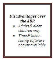 difference of 6.5 dB, after correction of which 94% of threshold estimates were within 15 dB. That is better than most estimates of adult ABR accuracy. Our study revealed that the test can be time-efficient with appropriately designed software that automates predictable manual tasks such as waveform manipulation: threshold estimation at three frequencies in both ears took an average of 20.6 minutes. With standard evoked potential software the test does take longer, principally because the user has to manually control the creation of grand averages, waveform manipulation, etc. Probably the most significant clinical limitation of the N1-P2 response as an audiological tool is its late maturation, extending into the late teenage years, though the technique remains viable in older children (Stapells, 2002). It is not appropriate for audiological use in infants, for whom the ABR (in its transient or 80 Hz ASSR guise) is a superior instrument because of earlier maturation of the relevant response generators. Devotees of the cortical response will know that the infant P1 (which is probably fused with the P2 response at that age) can be recorded at supra-threshold stimulus levels but that response cannot be used to reliably estimate auditory sensitivity.

Why Is This Response Almost Unknown?

The N1-P2 response has been criticized for its variability and susceptibility to the effects of subject drowsiness (Näätänen, 1992). Indeed, some texts on auditory evoked potentials appear to dismiss the technique as a viable audiological test (McPherson, 1966; Hall, 1992) perhaps because less than optimal test parameters have led to poor test performance. This is probably why the technique has not been widely used or taught, with tone burst ABR usually being the preferred method in many countries. The N1-P2 response does appear to be poor in a small proportion of individuals, with results overestimating the threshold by 20 dB or more. The resulting lack of clinical demand has stifled software development by equipment manufacturers. In contrast, Hyde (1997), Stapells (2002) and Martin et al. (2007) considered it to be the test of choice for threshold estimation of most older children and adults. Interestingly, individuals exaggerating their audiometric thresholds often give better responses than honest subjects, especially for stimulus levels that are audible but below their volunteered thresholds. This is thought to be associated with heightened cortical arousal level for these stimuli, which are seen as a threat. As with the ABR, the accuracy of threshold prediction increases for individuals with a recruiting hearing loss, the steeper response input-output function seen in such cases yielding larger amplitude responses than non-recruiting or normally hearing individuals at stimulus levels just above their threshold. In some countries (e.g., the UK) the test is established by legal case law and government military pension schemes as the ultimate objective arbiter of hearing status.

N1-P2 Response Characteristics & the Practicalities of Recording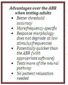

The response can be evoked by the relatively abrupt onset (or offset, or change) of an auditory stimulus. Frequency-specific stimuli are desirable for audiological applications and that usually means a tone burst. The amplitude of both ABR and CAEP responses are larger for stimuli with a more abrupt onset but a short rise time and duration limits frequency specificity. For the ABR, the universally agreed compromise between these competing requirements is a 2:1:2 cycle (rise/plateau/fall) tone burst. A rise time substantially longer than a couple of milliseconds "smears" the ABR in time because ABR latencies are so short. We can see that effect in the 500 Hz ABR: a rise time of 2 cycles at 500 Hz is 4 ms which is substantial compared to the Wave V latency, and we usually see a rather ill-defined ABR as a result. The much longer latencies of the N1-P2 complex give us the freedom to use longer stimulus rise times; a typical value being 10-20 ms. Stimulus plateau is typically 60 ms (see Frequency Conversion Table and Trial Settings section at the end of this document). By that time, the response either will or will not have been evoked so there is little merit in extending the duration of the stimulus beyond this value. One of the advantages of the N1-P2 response is therefore the almost ideal frequency specificity it provides, allowing steeply sloping or notched audiometric contours to be resolved. Unlike the ABR, the morphology of the N1-P2 response is every bit as clear for low frequencies as for high frequencies. Response amplitude does decline at frequencies above about 3 kHz but we found that threshold prediction at 8 kHz was no worse than at lower frequencies (Lightfoot & Kennedy, 2006; our study used stimuli of 1, 3 and 8 kHz).

In addition to the excellent frequency specificity and good threshold precision, other advantages over the ABR include testing the integrity of a greater proportion of the auditory nervous system and the capability to employ speech-based stimuli.

For clinical threshold estimation a single recording channel is sufficient, with a Cz positive electrode site (a high forehead site will give a significantly attenuated amplitude) and a mastoid (either right or left, or linked mastoids) negative electrode site. Ground is conventionally placed on the forehead. This set up is illustrated in Figure 1.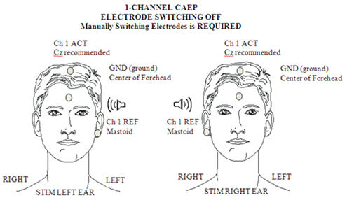



Figure 1. Electrode placement for 1-channel CAEP.

Filters of 1 Hz to 15 Hz provide the best signal to noise compromise when the response is used to estimate threshold; this is a much narrower bandwidth than one would use for research where waveform fidelity is important. The amplifier gain/artefact rejection setting should be such that incoming signals greater than about ±50 µV (e.g., 60%) are rejected. The choice of repetition rate is an interesting compromise: it takes about 10 seconds for the response to fully recover (Davis, Mast, Yoshie & Zerlin, 1966). A rate above 0.1 Hz will diminish the response amplitude, but faster stimulation allows more averaging and hence greater signal to noise ratio improvement per unit test time. A repetition rate of 0.5 to 1.0 stimuli per second is optimal. However, this means that the first few stimuli in an averaging sequence (preceded by silence) will evoke larger responses and as the averaging run continues the response amplitude will decline. Very long averaging runs are therefore counterproductive. At each stimulus level, typically two or three waveforms with 10 - 20 sweeps each are sufficient to identify a response at supra-threshold stimulus levels but 20 - 40 sweeps per waveform are usually needed close to threshold. Recording more than a single waveform allows us to assess response repeatability (by visual inspection and by computer correlation) and residual noise (as the average gap between replicates). For this process to be valid, the response should be stationary, i.e., not change with time. But we know that this response declines with time during an averaging run and can vary with the patient's level of arousal. These effects can be minimized in dedicated software by acquiring the 2 or 3 replicates pseudo-simultaneously or, less ideally, by manually ensuring that a silent period of at least 10 seconds separates the averaging runs. A recording epoch (time base) of 500 ms to 1000 ms is usual, the latter allowing some pre-stimulus activity to be recorded as an indication of background non-response electrical activity.

Unlike shorter latency responses which place high demands on muscle relaxation, CAEP subjects simply need to remain awake and reasonably alert during testing. This can readily be achieved by asking them to sit upright (not reclined) in a chair and browse a magazine or watch a silent video. Eye closure is to be avoided since this is associated with EEG alpha (8 - 12 Hz) activity which can contaminate the recording as well as increased drowsiness. Asking the subject to listen to or count the stimuli is unnecessary.

Response Identification

Although some objective assessment tools such as measurement of signal-to-noise ratio and cross-correlation are available on most evoked potential equipment, N1-P2 response identification (like ABR response identification) is usually based on subjective judgment by the audiologist and is therefore vulnerable to operator error or bias.

Figure 2 illustrates N1-P2 CAEPs at a number of stimulus levels. The stimulus was a 120 cycle plateau tone burst at 2 kHz with 20 cycle linear rise and fall times. See cortical protocol Trial Settings section at the end of this document.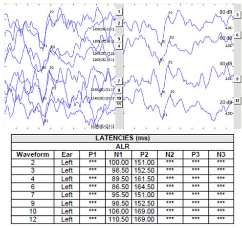



Figure 2. N1-P2 intensity series

In Figure 2 the left panel shows replicated responses; the right panel shows the grand averages of the replicates. The manner in which response amplitude and latency change as stimulus level is changed is, for frequency-specific stimuli, quite predictable though influenced by the extent of any loudness recruitment present. Responses at supra-threshold test levels, in combination with input-output (I/O) functions for the N1-P2 complex (see Lightfoot & Kennedy, 2006) can be helpful in the correct identification of near-threshold responses.

The appropriate identification of the lowest level at which a response is seen is only half of the threshold estimation process; the other is the highest level at which a response is absent. For the latter to be valid, not only must there be no obvious response but we also need to be sure that the recording conditions are sufficiently good to ensure that a small response is not obscured by residual noise. Note that there is an important distinction between not seeing an obvious response and being able to demonstrate that a response is absent. A maximum residual noise level criterion is therefore appropriate when defining response absence and for the N1-P2 response a value around 1.5 µV is reasonable for this purpose. One way of assessing the residual noise is by superimposing replicates and then visually estimating the average gap between them, across the entire recording window. At points where the waveforms cross, the gap is zero (obviously) whereas at other latencies the gap will be a maximum. At stimulus levels where there is no obvious response present and the noise estimate is acceptably low, one can state with reasonable confidence that this stimulus level is below threshold. Of course it is possible that some recordings may fail to meet the acceptance criteria of either the response presence or response absence status. Examples include "probable" responses that have a signal-to-noise ratio below an acceptable value and "probably absent" responses where the residual noise level is above an acceptable value. Such waveforms must be graded as inconclusive and though tempting, must not be allowed to contribute to the process of threshold definition. This is equally true of ABR responses, though sadly, it is common for this issue to be overlooked in clinical practice. Additional averaging, leading to a lower residual noise, is the most obvious means of resolving inconclusive waveforms.

Case Study: Medico-legal Noise Trauma

Figure 3 is the audiogram of a 36-year-old telephonist who wore her earpiece in the right ear. Her main complaint was that of right-sided continual hissing tinnitus following an incident in which her right ear received a very high level noise for a few seconds during equipment malfunction. She reported her hearing as reasonably good bilaterally (audiometric thresholds were ≤20 dB HL on the left). The authenticity of the 6 kHz threshold on the right (and by inference, the existence of the tinnitus) was questioned by the defendant and CAEPs were commissioned.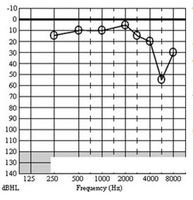



Figure 3. Case study - audiogram

Figures 4 & 5 are the CAEP waveforms at 4 kHz & 6 kHz respectively. The dotted vertical line denotes stimulus onset. Full details of test parameters and procedure are given in Lightfoot and Kennedy (2006). The residual noise (RN) in each waveform is a function of the number of sweeps in each average and was calculated as the mean of the modulus of the differences between the sub-averages across the entire recording window. This is the same as the subjective noise estimation method suggested above. At the highest stimulus level in Figures 4 and 5, only 15 sweeps were used (bold lines, showing the grand average of the three sub-averages which were the result of only 5 sweeps each) since the response was clear even in the presence of a moderately high residual noise. At lower test levels the declining response amplitude leads to a declining signal-to-noise ratio (S/N) and 30 sweeps were used to obtain a lower RN and hence a good S/N. Here, S/N was calculated as the N1-P2 amplitude divided by RN. At the sub-threshold levels 45 sweeps were needed to obtain a sufficiently low noise floor to ensure the response was absent.

The author's system calculates the correlation between the sub-averages in the region of a suspected response (50 ms prior to where the system detects a potential N1 to 50 ms following a potential P2) and uses this correlation together with the S/N to derive a p-value (the likelihood of the response being spurious) for the response (Lightfoot, 2009). Note how in Figures 4 and 5 the p-values are very low for the supra-threshold responses, supporting the subjective visual interpretation that at these levels there are likely genuine responses. At 4 kHz there are unequivocal responses at 60, 40 and 30 dB HL whilst at 20 dB HL the objective measures suggest there is no response. Subjectively it is tempting to grade this as a "possible response" but we must resist! The minor bump suggesting a P2 is predominantly from only one of the three sub-averages and is therefore probably just residual noise.

We employ a rule whereby if the amplitude of the lowest level response is>3 µV (>5 µV at 1 kHz or below) then the threshold is taken as 5 dB below this level. The CAEP result therefore predicts a threshold of 25 dB HL at 4 kHz, validating the audiogram. The 6 kHz responses suggest a threshold of 55 dB HL, in complete agreement with the behavioral audiogram. This is an example of recruitment sharpening our precision.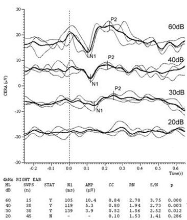



Figure 4. Right ear 4 kHz CAEPs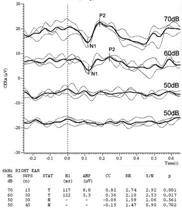



Figure 5. Right ear 6 kHz CAEPs

In this case, CAEP testing was able to confirm the presence of a fairly tight notch in the audiogram. Recall that a stimulus rise time of 10 ms was used. At 6 kHz that represents 60 cycles, not the 2 cycles used in ABR. It is unsurprising that this stimulus is sufficiently frequency-specific to probe such audiometric notches.

Trial Settings and Frequency Conversion Table

Figure 6 shows the cortical protocol trial settings. Artifact rejection is set at 60% = +/- 50 uV. The recommended Display Scale is 3.00 uV.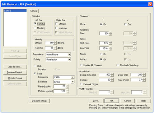



Figure 6. Cortical protocol test settings.

Figure 7 shows the milliseconds to cycles conversion table at 10 ms (rise/fall) , 20 ms (rise/fall) and 60 ms (plateau).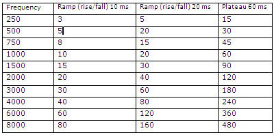



Figure 7. Milliseconds to cycles conversion table.

Closing Remarks

The N1-P2 CAEP is not without imperfections and limitations (most important is its inapplicability to infants) but it is a valuable component of the audiologist's toolbox. Its success in hearing threshold estimation lies in the use of appropriate test parameters, efficient procedure, and rigorous interpretation. If there is sufficient demand, I hope that equipment manufacturers will develop and provide labor & time-saving software - so let them know!

References

Davis, H., Mast, T., Yoshie, N., & Zerlin, S. (1966). The slow response of the human cortex to auditory stimuli: Recovery process. Electroenceph Clin Neurophysiol, 21,105-113.

Hall, J.W. (1992). Handbook of auditory evoked responses. Boston: Allyn and Bacon.

Hyde, M. (1997). The N1 response and its applications. Audiol Neurootol, 2, 281-307.

Lightfoot, G., & Kennedy, V. (2006). Cortical electric response audiometry hearing threshold estimation: Accuracy, speed and the effects of stimulus presentation features. Ear Hear, 27(5), 443-456.

Lightfoot, G. (2009). Objective detection of the cortical N1-P2 response using signal to noise ratio. Oral presentation at the XXI Biennial Symposium of the International Evoked Response Study Group, Rio de Janeiro, Brazil.

Martin, B.A., Tremblay, K.L., & Stapells, D.R. (2007). Principles and applications of cortical auditory evoked potentials. In R.F. Burkard, M. Don, & J.J. Eggermont (Eds.), Auditory Evoked Potentials (pp. 482 - 507). Baltimore: Lippincott Williams and Wilkins.

McPherson, D.L. (1996). Late Potentials of the Auditory System. San Diego: Singular.

Näätänen, R. (1992). Attention and Brain Function. Hillsdale. NJ: Lawrence Erlbaum Associates.

Stapells, D. (2002). Cortical event-related potentials to auditory stimuli. In J. Katz (Ed.), Handbook of Clinical Audiology (5th Ed). Philadelphia: Lippincott Williams & Wilkins.